Int'l MacroEcon 笔记

本文是国际宏观经济学的笔记，教材是「International Macroeconomics: A Modern Approach」

L1 - Introduction

Positive vs. Normative

• Positive economics: How does the world work?
• Normative economics: How should the world work?

Balance of Payments Accounts

Current Account (CA)

• CA records exports and imports of G&S, int'l receipts and payments of income.
• (+) -> exports, income receipts
• (-) -> imports, income payments

Current Account Balance

• Trade Balance
  • Merchandise Trade Balance: NX of goods
  • Service Balances: NX of services
• Income Balance
  • Net Investment Income: interests, diidends
  • Net International Compensation to Employees: compensation to (domestic workers abroad - foreign workers)
• Net Unilateral Transfers
  • Personal Remittances
  • Government Transfers

Financial Account (FA)

• changes in a country's net foreign asset position.
• (+) -> Sell assets to foreigners
• (-) -> buy assets from abroad

Financial Account Balance

• Increase in Foreign-Owned Assets in Home Country - Increase in Home-Owned Assets Abroad
• Assets include: Securities, Currencies, Bank loans, Foreign direct investment (FDI)

Fundamental Balance-of-Payments Identity

• CA Balance = -(FA Balance)

Capital Account

• 3rd account besides CA and FA
• Records international transfers of financial capital
  • debt forgiveness
  • migrants' transfers
• Not discussed in this course

CA/FA Balance Practice

(a) An Australian resident buys a smartphone from South Korea for $500

Answer: CA = -500, FA = +500 (import goods)

(b) An Italian friend comes to Australia and stays at Plaza Hotel paying for $400 with his Italian VISA card.

Answer: CA = +400, FA = -400 (export serices)

(c) Australian government send $700 medicines to an African country affected by epidemic.

Answer: CA = 700 - 700 = 0, FA = 0 (unilateral transfer)

Reason: CA +700 (export goods); CA -700 (gives up receiving money)

(d) An Australian resident purchases shares from FIAT Italy with AUD.

Answer: CA = 0; FA = -400 + 400 = 0

Reason: FA -400 (buy shares from abroad); FA +400 (sell AUD to FIAT Italy)

Net International Investment Position (NIIP)

NIIP = A - L

• A -> foreign assets held by home residents
• L -> home assets held by foreigners

A CA deficit implies that the country has to

• Reduce A (int'l asset position)
• Increase L (int'l liability position)

Valuation changes: prices of financial instruments (currency, stock, bond) can change

ΔNIIP = CA + Valuation Changes

Valuation Changes Example

International assets:

• 25 shares of Italian carmaker Fiat
• 2 € per share
• 2 AUD per €

International liabilities:

• 80 Australian bonds held by foreigners
• 1 AUD per unit

NIIP = A - L = 25 · 2 · 2 - 80 · 1 = 20 AUD

【Event 1】Euro depreciates to 1 AUD per €

• NIIP = A - L = 25 · 2 · 1 - 80 = -30 AUD

【Event 2】Share price of Fiat increases to 7 € per share

• NIIP = A - L = 25 · 7 · 1 - 80 = 95 AUD

NIIP Practice

The question is about balance of payments of US. Exchange rate is EUR/USD = 1.5

Question 1

• US starts 2023 with 100 shares of Volkswagen (1 EUR/share)
• RW holds 200 units of US government bonds (2 USD/unit)
• Calculate $NIIP^{US}$

Answer 1

• $A^{US}$ = 100 · 1 · 1.5 = 150 USD
• $L^{US}$ = 200 · 2 = 400 USD
• $NIIP^{US}=A^{US}-L^{US}$ = -250 USD

Question 2

• US 2023 exports: Toys (7 USD)
• US 2023 imports: Shirts (9 EUR)
• Rate of return on Volkswagen shares: 5%
• Rate of return on Outlandian bonds: 1%
• US residents received 3 EUR from relatives living abroad
• US government donated 4 USD to a hospital in Africa
• Calculate TB, NII, Net Unilateral Transfers, CA, NIIP

Answer 2

• TB = 7 - 1.5 · 9 = -6.5 USD
• NII (Income Balance) = 0.05 · 100 · 1.5 - 0.01 · 400 = 3.5 USD
• Net Unilateral Transfers = 3 · 1.5 - 4 = 0.5 USD
• Current Account = -6.5 + 3.5 + 0.5 = -2.5 USD
• NIIP = -250 - 2.5 = -252.5 USD

L2.1 - NIIP-NII-Paradox

If no valuation changes: $NIIP_{t}=(CA_{t}+\dots+CA_{1})+NIIP_{0}$

NII and NIIP in the US

• NIIP < 0 (largest external debtor)
• NII > 0 (receives more investment income)

Dark Matter Hypothesis

NIIP > 0, but the BEA fails to account for all of it

• BEA -> Bureau of Economic Analysis (US)

Hypothesis:

• U.S. FDI contains intangible capital (e.g. brand capital)
• intangible capital not reflected in NIIP, but recorded in NII
• Therefore, NIIP < 0 and NII > 0

Validation:

• TNIIP (true NIIP) = NIIP + Dark Matter
  • NIIP = observed NIIP (-$11.1T in 2020)
  • NII = net investment income ($0.1909T in 2020)
  • r = interest rate on net foreign assets (0.05)
  • NII = r · TNIIP
• TNIIP = NII / r = $3.818T
• Dark Matter = TNIIP - NIIP = $14.9T
• It's unlikely for $14.9T to go unnoticed by BEA

Return Differentials

Hypothesis:

• A -> risky, high-return assets (foreign equity and FDI)
• L -> safer, low-return assets (US government bonds, T-bills)
• Let: $r^{A}$ (return on A), $r^{L}$ (return on L)
• If interest rate differential $r^{A}-r^{L}\gt 0$, then NIIP < 0 and NII > 0

Validation:

• $NII=r^{A}A-r^{L}L$
  • A = $32.2T
  • L = $46.3T
  • $r^{L}$ = 0.37%
  • NII = $0.1909T
• Therefore, $r^{A}$ = 1.12%, $r^{A}-r^{L}$ = 0.75%
• This is more plausible than Dark Matter Hypothesis

Flipped NIIP-NII-Paradox

$NIIP^{US}=A^{US}-L^{US}=L^{RW}-A^{RW}=-NIIP^{RW}$

$NII^{US}=r^{A}A^{US}-r^{L}L^{US}=r^{A}L^{RW}-r^{L}A^{RW}=-NII^{RW}$

The rest of the world (RW) must experience a flipped paradox: $NIIP^{RW}$ > 0 and $NII^{RW}$ < 0

• e.g. China

L2.2 - CA Sustainability

CA surplus and deficit

• CA surplus (pay < receive): CN, DE, JP
• CA deficit (pay > receive): US, UK

Perpetual Trade Balance (TB)

• NO: initial NIIP < 0 (debtor)
  • need TB surplus to service its debt
• YES: initial NIIP > 0
  • finance the deficit with interests from net investments abroad

Perpetual TB Deficit Analysis

Rules:

• The economy lasts for only two periods, periods 1 and 2.
• The interest rate r on investments held for one period is exogenously given
• Further assumptions:
  • no international compensation to employees
  • no unilateral transfers
  • no valuation changes of assets in this world

Notation:

• $TB_{1}$: Trade balance in period 1
• $CA_{1}$: Current account balance in period 1
• $B_{0}$: The country's NIIP at the beginning of period 1
• $B_{1}$: The country's NIIP at the end of period 1

From definition:

• $CA_{1}=TB_{1}+rB_{0}$ (CA balance definition, Assumptions 1 & 2)
• $CA_{1}=B_{1}-B_{0}$ (ΔNIIP definition, Assumption 3)

We can dirive:

• $B_{1}=(1+r)B_{0}+TB_{1}$
• $B_{2}=(1+r)B_{1}+TB_{2}$

We can get $B_{0}=\frac{B_{2}}{(1+r)^{2}}-\frac{TB_{1}}{(1+r)}-\frac{TB_{2}}{(1+r)^{2}}$

Transversality Condition

• Let T denote the terminal date of the economy, then $B_{T} = 0$
• If $B_{T} \lt 0$, RW can't collect debt from the country
• If $B_{T} \gt 0$, the country can't collect debt from RW
• In this analysis, $B_{2} = 0$

Given Transversality Condition:

• $B_{0}=-\frac{TB_{1}}{(1+r)}-\frac{TB_{2}}{(1+r)^{2}}$
• If $B_{0} \gt 0$, it's possible to have $TB_{1} \lt 0$ and $TB_{2} \lt 0$
• If $B_{0} \lt 0$, it must be $TB_{1} \gt 0$ or $TB_{2} \gt 0$

Since $NIIP^{US} \lt 0$ currently, it will have to run TB surplus in the future.

Perpetual CA Deficit Analysis

Same rules from Perpetual TB Deficit Analysis

We had already derived:

• $CA_{1}=B_{1}-B_{0}$ (ΔNIIP definition, Assumption 3)
• $CA_{2}=B_{2}-B_{1}$ (same reasoning)

We can get:

• $B_{0}=-CA_{1}-CA_{2}+B_{2}$

Transversality Condition ($B_{2}=0$):

• $B_{0}=-CA_{1}-CA_{2}$
• If $B_{0} \gt 0$, it's possible to have $CA_{1} \lt 0$ and $CA_{2} \lt 0$
• If $B_{0} \lt 0$, it must be $CA_{1} \gt 0$ or $CA_{2} \gt 0$

Since $NIIP^{US}$ < 0 currently, it will have to run CA surplus in the future.

Four ways of viewing CA

CA as Changes in NIIP

• $CA_{t}=B_{t}-B_{t-1}$
• Notations:
  • $CA_{t}$: The country's current account in period t
  • $B_{t}$: The country's NIIP at the end of period t
• If $CA_{t} \lt 0$, NIIP falls
• If $CA_{t} \gt 0$, NIIP rises

CA as Reflections of TB and NII

• $CA_{t}=TB_{t}+rB_{t-1}$
• Notation:
  • $TB_{t}$: The country's trade balance in period t
  • $r$: The interest rate on investments held for one period
• This is the original definition of CA

CA as the Gap Between Savings and Investment

• $CA_{t}=S_{t}-I_{t}$

CA as the Gap between National Income and Domestic Absorption

• $CA_{t}=Y_{t}-A_{t}$
• Note: domestic absorption $A_{t}\equiv C_{t}+I_{t}+G_{t}$

Perpetual TB Deficits (Infinite Economy)

Time periods $t = 1, 2, \ldots$

The interest rate $r (> 0)$ on investments held for one period is constant over time

As before $B_1 = (1 + r)B_0 + TB_1$, and thus $B_0 = \frac{B_1}{1 + r} - \frac{TB_1}{1 + r}$

Generalizing, for all $t \geq 1$, $B_{t-1} = \frac{B_t}{1 + r} - \frac{TB_t}{1 + r}$

Therefore, repeatedly using (13), for all $T \geq 1$,

$B_0 = \frac{B_1}{1 + r} - \frac{TB_1}{(1 + r)}$

$B_0 = \frac{B_2}{(1 + r)^2} - \frac{TB_1}{1 + r} - \frac{TB_2}{(1 + r)^2}$

$B_0 = \frac{B_3}{(1 + r)^3} - \frac{TB_1}{1 + r} - \frac{TB_2}{(1 + r)^2} - \frac{TB_3}{(1 + r)^3}$

$B_0 = \frac{B_T}{(1 + r)^T} - \frac{TB_1}{1 + r} - \ldots - \frac{TB_T}{(1 + r)^T}$ (14)

Assuming the transversality condition: $\lim_{T \to \infty} \frac{B_T}{(1 + r)^T} = 0$

Taking limits on both sides of (14) yields: $B_0 = - \sum_{t=1}^{\infty} \frac{TB_t}{(1 + r)^t}$ (15)

We obtain the same conclusion as in the 2-period case:

• If $B_0 > 0$, it is possible (but not necessary) to have $TB_t < 0$ for all $t \geq 1$
• If $B_0 < 0$, we must have $TB_t > 0$ for some $t \geq 1$

A country can run a perpetual trade deficit only if the country has positive initial NIIP

Perpetual CA Deficits (Infinite Economy)

We will show that in contrast to finite horizon economies, in infinite horizon economies perpetual CA deficits can be possible even if the country has a negative initial NIIP

We give the example of an economy that is growing and dedicates a growing amount of resources to pay interest on its external debt

Suppose that:

• $B_0 < 0$
• $r > 0$
• $\alpha \in (0, 1)$
• $TB_t = -\alpha rB_{t-1}$ (whenever $B_{t-1} < 0$ the country generates a TB surplus that suffices to cover a fraction $\alpha$ of its interest obligations)

Then $B_t = (1 + r)B_{t-1} + TB_{t-1} = (1 + r - \alpha r) B_{t-1} < 0, \text{ for all } t \geq 1$ (16)

• $(1 + r - \alpha r) > 0$
• NIIP is negative in all periods

Moreover, $CA_t = rB_{t-1} + TB_t = r(1 - \alpha)B_{t-1} < 0, \text{ for all } t \geq 1$

• $r(1 - \alpha) > 0$
• $B_{t-1} < 0$
• the country runs a perpetual CA deficit

(16) implies that for all $t \geq 1, B_t = (1 + r - \alpha r)^t B_0$

Thus, the transversality condition is satisfied:

$\frac{B_t}{(1 + r)^t} = \left(\frac{1 + r - \alpha r}{1 + r}\right)^t B_0 \to 0$ as $t \to \infty$

For all $t \geq 1, TB_t = -\alpha rB_{t-1} = -\alpha r(1 + r - \alpha r)^{t-1} B_0 > 0$, therefore, the trade balance grows unboundedly over time

Since $TB_t = X_t - IM_t = Q_t - C_t - I_t - G_t = Q_t - A_t$ and $A_t = C_t + I_t + G_t \geq 0$, the GDP $Q_t$ must grow unboundedly over time, as well.

L3 - CA Determination

Optimal Intertemporal Allocation

• makes intertemporal consumption and saving decisions
• smoothes consumption over time by borrowing and lending

Intertemporal Budget Constraint

Rules:

• Two-period small open economy: periods 1 and 2
• The single consumption good in the economy is perishable
  • cannot be stored across periods
• The single asset traded in the financial market is a bond
  • measured in units of the consumption good
• There is a single representative household (HH) in the economy endowed with
  • $B_{0}$ units of the bond at the beginning of period 1
  • $Q_{1}$ units of the good in period 1
  • $Q_{2}$ units of the good in period 2
• Interest Rates:
  • $r_{0}$ for the initial bond holdings
  • $r_{1}$ for the bonds held at the end of period 1
• The HH can reallocate resources between periods by purchasing or selling bonds (via international financial market)
  • $B_{t}=NIIP$

The HH's budget constraint in period 1 is:

• $C_{1}+B_{1}=(1+r_{0})B_{0}+Q_{1}$
• Notations:
  • $C_{1}$ is consumption in period 1
  • $B_{1}$ is the amount of bonds held at the end of period 1

The HH's budget constraint in period 2 is:

• $C_{2}+B_{2}=(1+r_{1})B_{1}+Q_{2}$
• Note: $B_{2}=0$ (transversality condition)

By combining the above, we obtain the HH's intertemporal budget constraint. The intertemporal budget constraint describes the consumption paths $(C_{1}, C_{2})$ that the HH can (just) afford.

$C_{1}+\frac{C_{2}}{1+r_{1}} =(1+r_{0})B_{0}+Q_{1}+\frac{Q_{2}}{1+r_{1}}$ (Consumption Values = Initial Assets + Total Income Values)

The slope of the budget constraint is $-(1+r_{1})$

Utility and Indifference Curves

The utility function $U(C_{1}, C_{2})$ can be represented by indifference curves (ICs).

Common Utility Functions

• Logarithmic: $U(C_{1},C_{2})=\ln C_{1}+\ln C_{2}$
• Square-root: $U(C_{1},C_{2})={\sqrt{C_{1}}}+{\sqrt{C_{2}}}$
• Cobb-Douglas: $U(C_{1},C_{2})=(C_{1})^{\alpha}(C_{2})^{1-\alpha}$ where $(0\lt \alpha\lt 1)$

Properties of Indifference Curves

• ICs do not intersect
• ICs are downward sloping
  • True if more is better
• The right-upper ICs indicate higher levels of utility
• ICs have a bowed-in shape towards the origin (convex toward the origin)

Slope of Indifference Curves (MRS)

${\mathrm{MRS}}={\frac{U_{1}(C_{1},C_{2})}{U_{2}(C_{1},C_{2})}}$, where:

• $U_{1}(C_{1},C_{2})=\frac{\partial U(C_{1},C_{2})}{\partial C_{1}}$
• $U_{2}(C_{1},C_{2})=\frac{\partial U(C_{1},C_{2})}{\partial C_{2}}$

Slope of IC containing $(C_{1},C_{2})$ at $(C_{1},C_{2})$ is $-{\frac{U_{1}(C_{1},C_{2})}{U_{2}(C_{1},C_{2})}}$

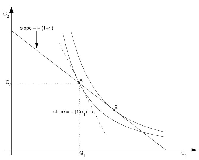
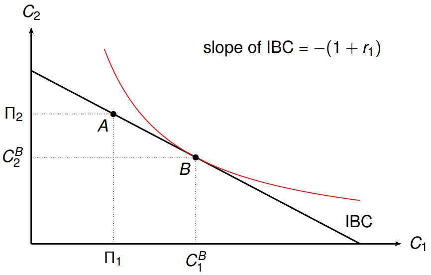
Optimal Intertemporal Allocation

The HH maximizes utility subject to the intertemporal budget constraint.

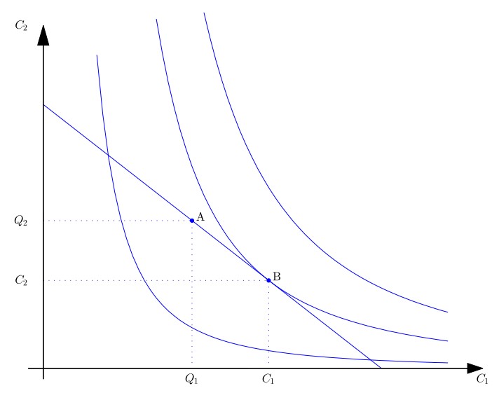
The optimal consumption path is point B.

At the optimal bundle $(C_{1},C_{2})$ the IC is tangent to the intertemporal budget constraint (IBC)

$-{\frac{U_{1}(C_{1},C_{2})}{U_{2}(C_{1},C_{2})}}=-(1+r_{1})$

or equivalently, $U_{1}(C_{1},C_{2})=(1+r_{1})U_{2}(C_{1},C_{2})$

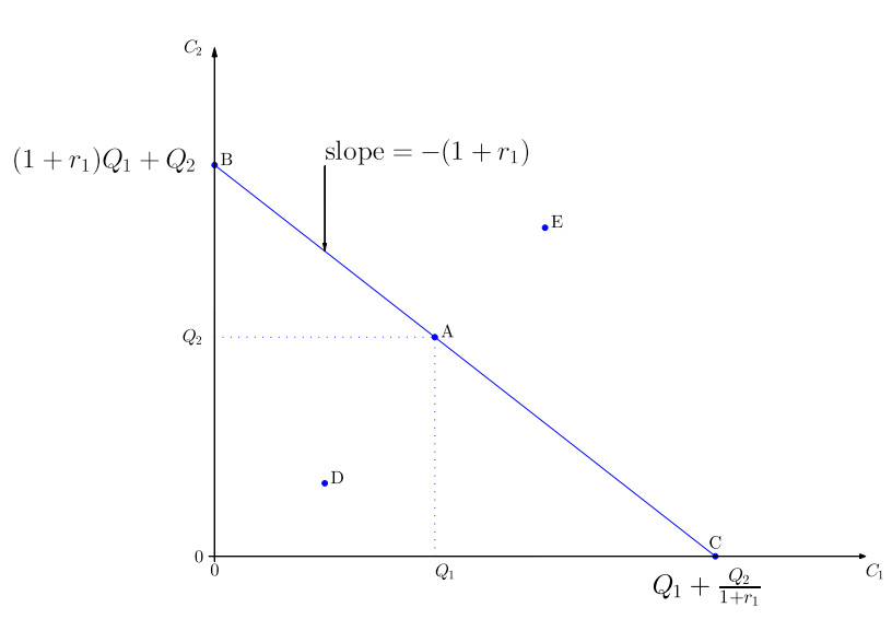
TB and CA in Equilibrium

Exogenously given are $r_{0}$, $B_{0}$, $r^{*}$, $Q_{1}$ and $Q_{2}$. An equilibrium is a consumption path $(C_{1},C_{2})$ and an interest rate $r_{1}$ such that:

• Feasibility of the intertemporal allocation
  • $C_{1}+\frac{C_{2}}{1+r_{1}} =(1+r_{0})B_{0}+Q_{1}+\frac{Q_{2}}{1+r_{1}}$
• Optimality of the intertemporal allocation
  • $U_{1}(C_{1},C_{2})=(1+r_{1})U_{2}(C_{1},C_{2})$
• Interest rate parity condition
  • $r_{1}=r^{*}$ (free capital mobility)

In this economy, $TB_{1}=Q_{1}-C_{1}$, $TB_{2}=Q_{2}-C_{2}$

And $CA_{1}=r_{0}B_{0}+TB_{1}$, $B_{1}=B_{0}+CA_{1}$, $CA_{2}=r_{1}B_{1}+TB_{2}$

Also, since we don't have investments in this economy $(I_{1}=I_{2}=0)$, $S_{1}=CA_{1}$, $S_{2}=CA_{2}$

Therefore, the HH's willingness to save determines the TB and CA

Temporary Output Shock

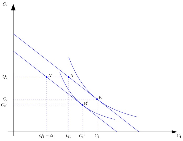
Budget Constraint and Optimal Allocation

• $C_{1}$ and $C_{2}$ are normal goods (their consumption increases with income)
• Output in Period 1 = $Q_{1}-\Delta$
• Output in Period 2 = $Q_{2}$
• A is the old and A′ the new endowment point
• B is the old and B′ the new optimal consumption path
• $C_{1}$ declines by less than ∆
• $TB_{1}$ deteriorates

Summary

• Relatively small effect on the consumption path $(C_{1},C_{2})$
• Temporary negative income shocks are smoothed out by borrowing from the rest of the world
• Generally, one should expect the borrowing to move the country's trade balance and current account significantly

Permanent Output Shock

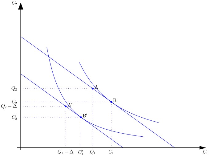
Budget Constraint and Optimal Allocation

• Output in Period 1 = $Q_{1}-\Delta$
• Output in Period 2 = $Q_{2}-\Delta$
• A is the old and A′ the new endowment point
• B is the old and B′ the new optimal consumption path
• $TB_{1}$ doesn't change much

Summary

• Relatively large effect on the consumption path $(C_{1},C_{2})$
• Generally, one should expect permanent negative income shocks to lead to similarly sized reductions in $C_{1}$ and $C_{2}$
• Generally, one should expect the country's trade balance and current account to not be much affected

Terms of Trade Shocks

Consider an economy which exports endowments of oil $(Q_{1},Q_{2})$ and imports food for consumption $(C_{1},C_{2})$

Then, the HH's budget constraints for period 1 and 2 are:

• $C_{1}+B_{1}=(1+r_{0})B_{0}+TT_{1}Q_{1}$
• $C_{2}=(1+r_{1})B_{1}+TT_{2}Q_{2}$

Terms of Trade (TT) are the relative price of exports in terms of imports:

• $TT_{1}=\frac{P_{1}^{X}}{P_{1}^{M}}$
• $TT_{2}=\frac{P_{2}^{X}}{P_{2}^{M}}$

With Terms of Trade Shocks, equlibrium would be:

• Feasibility of the intertemporal allocation (with $TT_1$ and $TT_2$)
  • $C_{1}+\frac{C_{2}}{1+r_{1}} =(1+r_{0})B_{0}+TT_1 Q_{1}+\frac{TT_2 Q_{2}}{1+r_{1}}$
• Optimality of the intertemporal allocation
  • $U_{1}(C_{1},C_{2})=(1+r_{1})U_{2}(C_{1},C_{2})$
• Interest rate parity condition
  • $r_{1}=r^{*}$ (free capital mobility)

Capital Controls

CA deficits are often viewed as bad for a country.

Assume the country's authority introduces a policy that prohibits borrowing, that is, requires $B_{1}$ ≥ 0

Result:

• The HH can't borrow
• The optimal allocation moves from B to A (IC is lower)
• Optimal consumption path changes to:
  • $C_{1}=Q_{1}$
  • $C_{2}=Q_{2}$
• $TB_{1}=TB_{2}=0$ $(TB_{t}=Q_{t}-C_{t})$

Logarithmic Utility Equilibrium

$U(C_{1},C_{2})=\ln C_{1}+\ln C_{2}$

Using derivatibe formula $\frac{d\ln(x)}{dx}=\frac{1}{x}$, we get:

$U_{1}(C_{1},C_{2})=\frac{\partial U(C_{1},C_{2})}{\partial C_{1}}=\frac{\partial(\ln C_{1}+\ln C_{2})}{\partial C_{1}}=\frac{1}{C_{1}}$

$U_{2}(C_{1},C_{2})=\frac{\partial U(C_{1},C_{2})}{\partial C_{2}}=\frac{\partial(\ln C_{1}+\ln C_{2})}{\partial C_{2}}=\frac{1}{C_{2}}$

Therefore, the equilibrium condition $U_{1}(C_{1},C_{2})=(1+r_{1})U_{2}(C_{1},C_{2})$ becomes ${\frac{1}{C_{1}}}=(1+r_{1}){\frac{1}{C_{2}}}$

From the above, we can derive $C_{2}=(1+r_{1})C_{1}$

By substituting into Feasibility of the intertemporal allocation, we get:

$C_{1}={\frac{1}{2}}[(1+r_{0})B_{0}+Q_{1}+{\frac{Q_{2}}{1+r_{1}}}]$

$C_{2}={\frac{1}{2}(1+r_{1})}[(1+r_{0})B_{0}+Q_{1}+{\frac{Q_{2}}{1+r_{1}}}]$

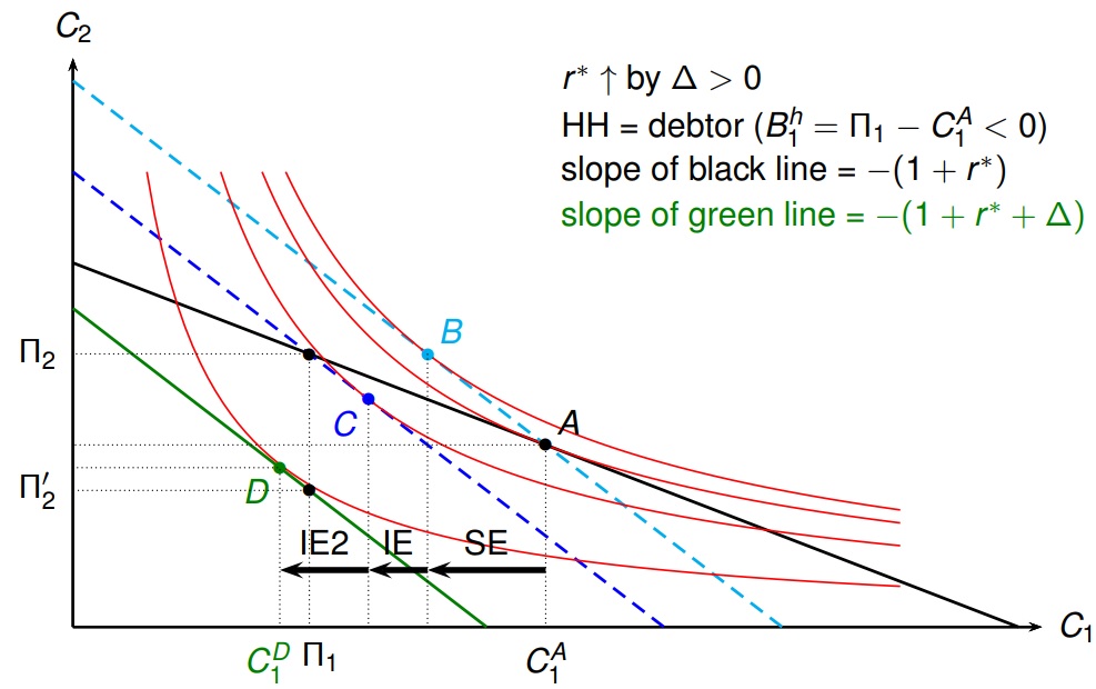
L4.1 - Int. R. Shocks & Tariffs in an Endowment Economy

World Interest Rate Shocks

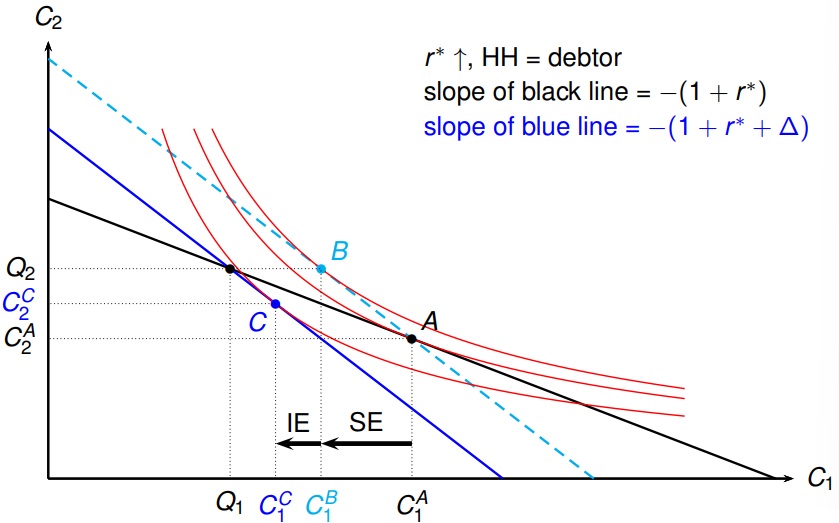
World interest rate increase from $r^{*}$ to $r^{*}+\Delta$

HH as debtor

HH as creditor

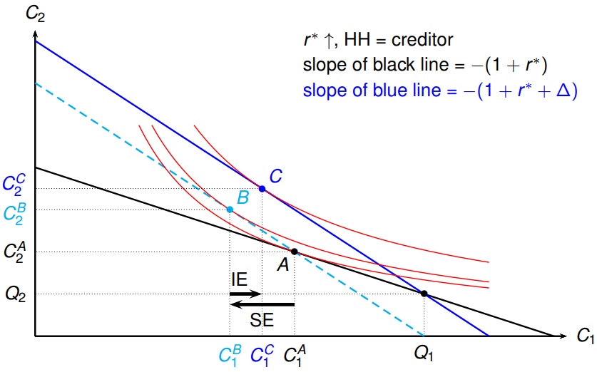
Substitution effect (SE)

• An increase in the interest rate makes $C_{1}$ relatively more expensive and $C_{2}$ relatively cheaper
• Change in period 1 consumption $C_{1}$ due to change in relative "price"
  • $A=(C_{1}^{A},C_{2}^{A})$ = originally optimal path
  • $B=(C_{1}^{B},C_{2}^{B})$ = path that is optimal given budget line that passes through A and has slope ${(-1+r^{*}+\Delta)}$
  • $SE=C_{1}^{B}-C_{1}^{A}\lt 0$
• Saving in period 1 becomes more attractive

Income effect (IE)

• Change in C1 due to change in purchasing power
  • $B=(C_{1}^{B},C_{2}^{B})$ = previous path
  • $C=(C_{1}^{C},C_{2}^{C})$ = new optimal path
  • $IE=C_{1}^{C}-C_{1}^{B}$
• $r^{*}$ ↑ has two opposing effects on HH's purchasing power
  • The HH can purchase more on a fixed budget since the “price” $\frac{1}{1+r^{*}}$ of $C_{2}$ falls
  • The present value $\frac{Q_{2}}{1+r^{*}}$ of endowment $Q_{2}$ decreases
• Netting these effect, $r^{*}$ ↑ makes
  • debtors (for whom $Q_{1}\lt C_{1}$ and thus $Q_{2}\lt C_{2}$) poorer
  • creditors (for whom $C_{1}\lt Q_{1}$ and thus $C_{2}\lt Q_{2}$) richer
• Since $C_{1}$ is a normal good
  • IE < 0 if purchasing power decreases (debtor)
  • IE > 0 if purchasing power increases (creditor)

TE (total effect) = SE + IE

Int. R. Shocks Summary

Overall, if the interest rate increases:

• If the country is a debtor $(Q_{1}\lt C_{1})$:
  • IE < 0 as budget line shift that determines IE is to the left.
  • TE = SE + IE < 0 as SE < 0 and IE < 0.
  • Therefore, HH's savings increase after the shock.
• If the country is a creditor $(Q_{1}\gt C_{1})$:
  • It remains a creditor after the interest rate rise (by a revealed preference argument).
  • IE > 0 as budget line shift that determines IE is to the right.
  • TE = SE + IE (> or <) 0 depending on which of SE and IE dominates.

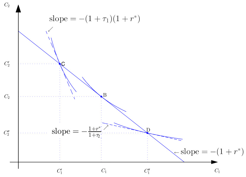
Import Tariffs

Given two-goods economy:

• exports endowments of oil $(Q_{1},Q_{2})$
• imports food for consumption $(C_{1},C_{2})$
• The HH treats $\tau_{t}$ and $L_{t}$ as exogeneously given

Assume that in each period t ∈ {1, 2}, the government

• imposes an import tariff $\tau_{t}\geq0$, and
• returns the revenue from $\tau_{t}$ via a lump-sum transfer $L_{t}$

Then, the HH's budget constraints for period 1 and 2 are:

$(1+\tau_{1})C_{1}+B_{1}=(1+r_{0})B_{0}+TT_{1}Q_{1}+L_{1}$

$(1+\tau_{2})C_{2}=(1+r_{1})B_{1}+TT_{2}Q_{2}+L_{2}$

HH's intertemporal budget constraint:

$(1+\tau_{1})C_{1}+\frac{(1+\tau_{2})C_{2}}{1+r_{1}}=(1+r_{0})B_{0}+TT_{1}Q_{1}+L_{1}+\frac{TT_{2}Q_{2}+L_{2}}{1+r_{1}}$

Slope: $[-\frac{1+\tau_{1}}{1+\tau_{2}}(1+r_{1})]$

The optimality condition (tangency of IC and IBC) becomes $U_{1}(C_{1},C_{2})=\frac{1+\tau_{1}}{1+\tau_{2}}(1+r_{1})U_{2}(C_{1},C_{2})$

• If τ1 = τ2, then there is no change from τ1 = τ2 = 0.
• If τ1 > τ2, then $C_{1}$ becomes relatively more expensive and, assuming diminishing marginal utilities, $C_{1}$ ↓ and $C_{2}$ ↑.
• If τ1 < τ2, then $C_{1}$ becomes relatively cheaper and, assuming diminishing marginal utilities, $C_{1}$ ↑ and $C_{2}$ ↓.

Import Tariffs Equilibrium

Exogenously given are $r_{0}$, $B_{0}$, $r^{*}$, $Q_{1}$, $Q_{2}$, $\tau_{1}$, and $\tau_{2}$.

An equilibrium is a consumption path $(C_{1},C_{2})$ and an interest rate $r_{1}$ such that:

• Feasibility of the intertemporal allocation
  • $C_{1}+\frac{C_{2}}{1+r_{1}} =(1+r_{0})B_{0}+TT_{1}Q_{1}+\frac{TT_{2}Q_{2}}{1+r_{1}}$
• Optimality of the intertemporal allocation
  • $U_{1}(C_{1},C_{2})=\frac{1+\tau_{1}}{1+\tau_{2}}(1+r_{1})U_{2}(C_{1},C_{2})$
• Interest rate parity condition
  • $r_{1}=r^{*}$ (free capital mobility)

Import Tariffs and TB

Question: Does an increase in import tariffs reduce imports and therefore improve TB?

$TB_{1}=TT_{1}Q_{1}-C_{1}$

An increase in import tariffs leads to

• TB ↑ if (present import tariff > expected future import tariff)
• TB - if (present import tariff = expected future import tariff)
• TB ↓ if (present import tariff < expected future import tariff)

Additional observation:

• In our model, $\tau_{1}\neq\tau_{2}$ leads to lower welfare than $\tau_{1}=\tau_{2}=0$ (no import tariffs)
• $\tau_{1}\neq\tau_{2}$ distorts the HH's optimal intertemporal allocation

L4.2 - CA Determination in a Production Economy

Now we introduce a representative firm in the economy, and firm's decision also significantly affects TB and CA.

Rules:

• Two-period small open economy: periods 1 and 2
• The single consumption good is perishable
• The single asset traded in the financial market is a bond (measured in units of the consumption good)
• There is a representative household (HH) endowed with $B_{0}^{h}$ units of the bond at the beginning of period 1
• There is a representative firm. The household owns the firm and obtains the firm's profits
  • $\Pi_{1}$ in period 1
  • $\Pi_{2}$ in period 2
• Interest Rates:
  • $r_{0}$ for the initial bond holdings
  • $r_{1}$ for the bonds held at the end of period 1

Firm

What does the firm do?

• makes investments in period $t$ that lead to output in $t + 1$
• finances its investments in period $t$ by issuing debt in $t$

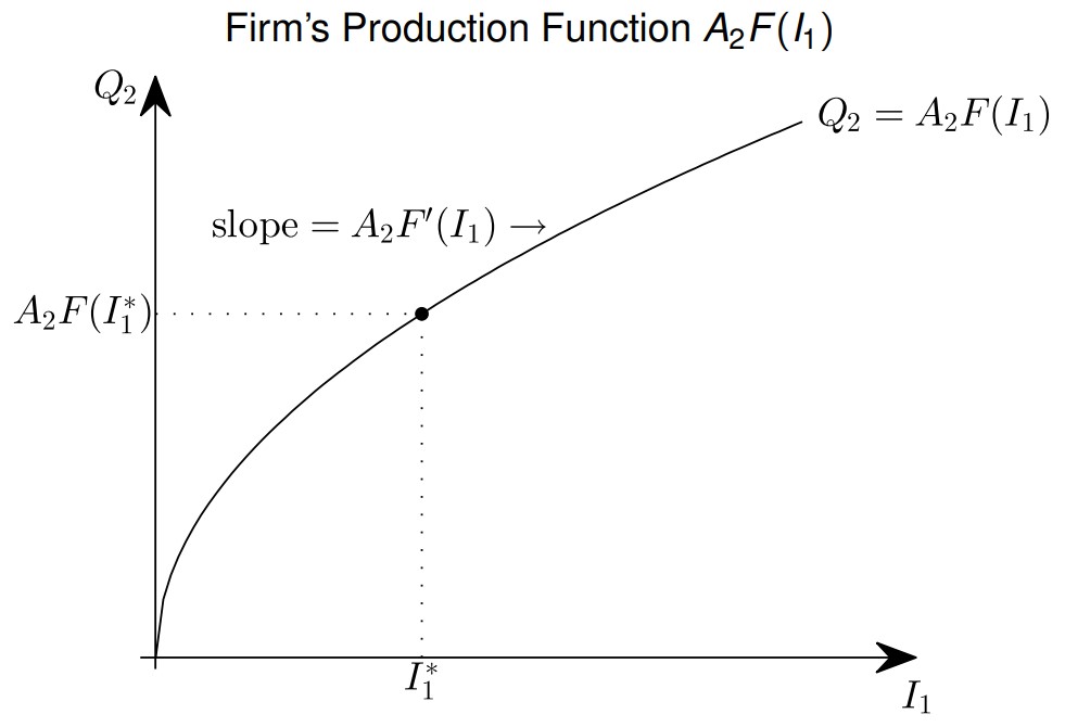
Firm's Production Function

• ${Q}_{1}=A_{1}F(I_{0})$
• ${Q}_{2}=A_{2}F(I_{1})$
• Notations:
  • $F$ is a function
  • $A_{t}\gt 0\ (t=1,2)$ are technology parameters
  • $I_{0}$ - investment in period 0 and exogeneously given
  • $I_{1}$ - investment in period 1 and chosen by the firm

Firm's Debt

• The firm issues debt $D_{t}^{f} (t=1,2)$
• $D_{0}^{f}=I_{0}$ (exogenous; to be repaid in period 1)
• $D_{1}^{f}=I_{1}$ (to be repaid in period 2)

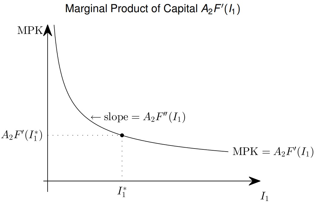
Production Function (MPK and MCK)

The firm chooses $I_{1}$ by maximizing profits

$\Pi_{2}=A_{2}F(I_{1})-(1+r_{1})D_{1}^{f} (\mathrm{where}\ D_{1}^{f}=I_{1})$

or $\Pi_{2}(l_{1})=A_{2}F(I_{1})-(1+r_{1})I_{1}$

The first-order condition for profit maximization is $\Pi_{2}^{\prime}(I_{1})=0$

Therefore, $0=A_{2}F^{\prime}(I_{1})-(1+r_{1})$

Thus, we have Optimal Investment Condition (MPK = MCK)

• $A_{2}F^{\prime}(I_{1})=(1+r_{1})$
• Marginal Product of Capital (MPK): ${\frac{d[A_{2}F(I_{1})]}{d I_{1}}}=A_{2}F^{\prime}(I_{1})$
• Marginal Cost of Capital (MCK): $(1+r_{1})$

We assume that F has the following properties:

• $F(0) = 0$
• Positive MPK: $F^{\prime}(l)=\frac{d F(I)}{dI}\gt 0$ for all $I\gt 0$
• Diminishing MPK: $F^{\prime\prime}(l)=\frac{d F^{\prime}(I)}{dI}\lt 0$ for all $I\gt 0$
• $\lim_{I \to 0}F^{\prime}(I)=\infty$ and $\lim_{I \to \infty}F^{\prime}(I)=0$
• The above properties guarantee:
  • the optimal investment condition has a unique solution
  • unique solution also maximizes profit
• Example: $F(I)={\sqrt{I}}$

Firm's Optimal Investment Decision

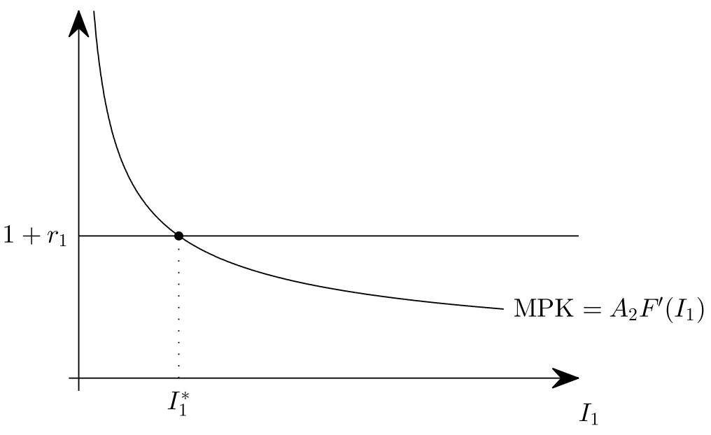
The firm chooses $I_{1}$ so that $A_{2}F^{\prime}(I_{1})=(1+r_{1})$

Household

Since the HH owns the firm, it receives the latter's profits:

• $\Pi_{1}=A_{1}F(I_{0})-(1+r_{0})D_{0}^{f}$
• $\Pi_{2}=A_{2}F(I_{1})-(1+r_{1})D_{1}^{f}$

The HH's budget constraint in period 1 is: $C_{1}+B_{1}^{h}=(1+r_{0})B_{0}^{h}+\Pi_{1}$

The HH's budget constraint in period 2 is: $C_{2}+B_{2}^{h}=(1+r_{1})B_{1}^{h}+\Pi_{2}$

Assume transversality condition $B_{2}^{h}=0$

From HH's budget constraint above, we obtain the HH's intertemporal budget constraint:

$C_{1}+\frac{C_{2}}{1+{r_{1}}}=(1+r_{0})B_{0}^{h}+\Pi_{1}+\frac{\Pi_{2}}{1+{r_{1}}}$

Economy's net foreign asset positions:

• $B_{0}=B_{0}^{h}-D_{0}^{f}$
• $B_{1}=B_{1}^{h}-D_{1}^{f}$
• Notations:
  • $B_{t}$: NIIP
  • $B_{t}^{h}$: Domestic Supply
  • $D_{t}^{f}$: Domestic Demand

By combining all the above, we obtain the economy's intertemporal resource constraint:

Steps

$C_{1}+\frac{C_{2}}{1+{r_{1}}}=(1+r_{0})(B_{0}+D_{0}^{f})+\Pi_{1}+\frac{\Pi_{2}}{1+{r_{1}}}$

$C_{1}+\frac{C_{2}}{1+{r_{1}}}=(1+r_{0})(B_{0}+D_{0}^{f})+[A_{1}F(I_{0})-(1+r_{0})D_{0}^{f}]+\frac{A_{2}F(I_{1})-(1+r_{1})D_{1}^{f}}{1+{r_{1}}}$

$C_{1}+\frac{C_{2}}{1+{r_{1}}}=(1+r_{0})(B_{0}+D_{0}^{f})+A_{1}F(I_{0})-(1+r_{0})D_{0}^{f}+\frac{A_{2}F(I_{1})}{1+{r_{1}}}-D_{1}^{f}$

$C_{1}+\frac{C_{2}}{1+{r_{1}}}+D_{1}^{f}=(1+r_{0})(B_{0}+D_{0}^{f}-D_{0}^{f})+A_{1}F(I_{0})+\frac{A_{2}F(I_{1})}{1+{r_{1}}}$

$C_{1}+\frac{C_{2}}{1+{r_{1}}}+D_{1}^{f}=(1+r_{0})B_{0}+A_{1}F(I_{0})+\frac{A_{2}F(I_{1})}{1+{r_{1}}}$

$C_{1}+\frac{C_{2}}{1+{r_{1}}}+I_{1}=(1+r_{0})B_{0}+A_{1}F(I_{0})+\frac{A_{2}F(I_{1})}{1+r_{1}}$

Equilibrium

Exogenously given are $r_{0}$, $B_{0}^{h}$, $r^{*}$, $I_{0}$, $D_{0}^{f}$, $A_{1}$ and $A_{2}$.

An equilibrium is $(C_{1},C_{2},I_{1},r_{1})$ such that:

• Feasibility of the intertemporal allocation
  • $C_{1}+\frac{C_{2}}{1+{r_{1}}}+I_{1}=(1+r_{0})B_{0}+A_{1}F(I_{0})+\frac{A_{2}F(I_{1})}{1+r_{1}}$
• Optimality of the intertemporal allocation
  • $U_{1}(C_{1},C_{2})=(1+r_{1})U_{2}(C_{1},C_{2})$
• Interest rate parity condition
  • $r_{1}=r^{*}$
• Optimal investment condition
  • $A_{2}F^{\prime}(I_{1})=(1+r_{1})$

Positive Productivity Shocks

Positive Anticipated Future Productivity Shock: Assume $\Delta\gt 0$ and that the period 2 technology parameter changes to $A_{2}^{\prime}=A_{2}+\Delta$, while $A_{1}$ remains unchanged

Firm's Decision

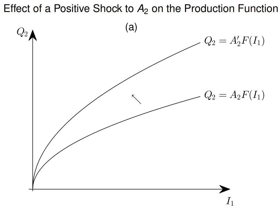
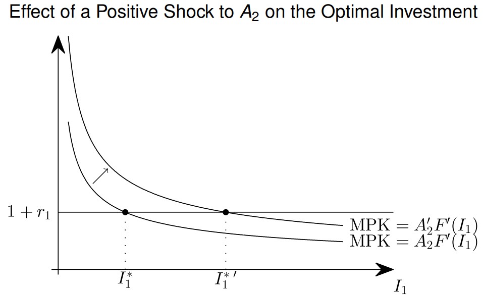
Productivity shocks affect the firm's optimal investment

• Positive shock: $I_{1}$ ↑, output ↑, $\Pi_{2}$ ↑
• Negative shock: $I_{1}$ ↓, output ↓, $\Pi_{2}$ ↓

Household's Reaction

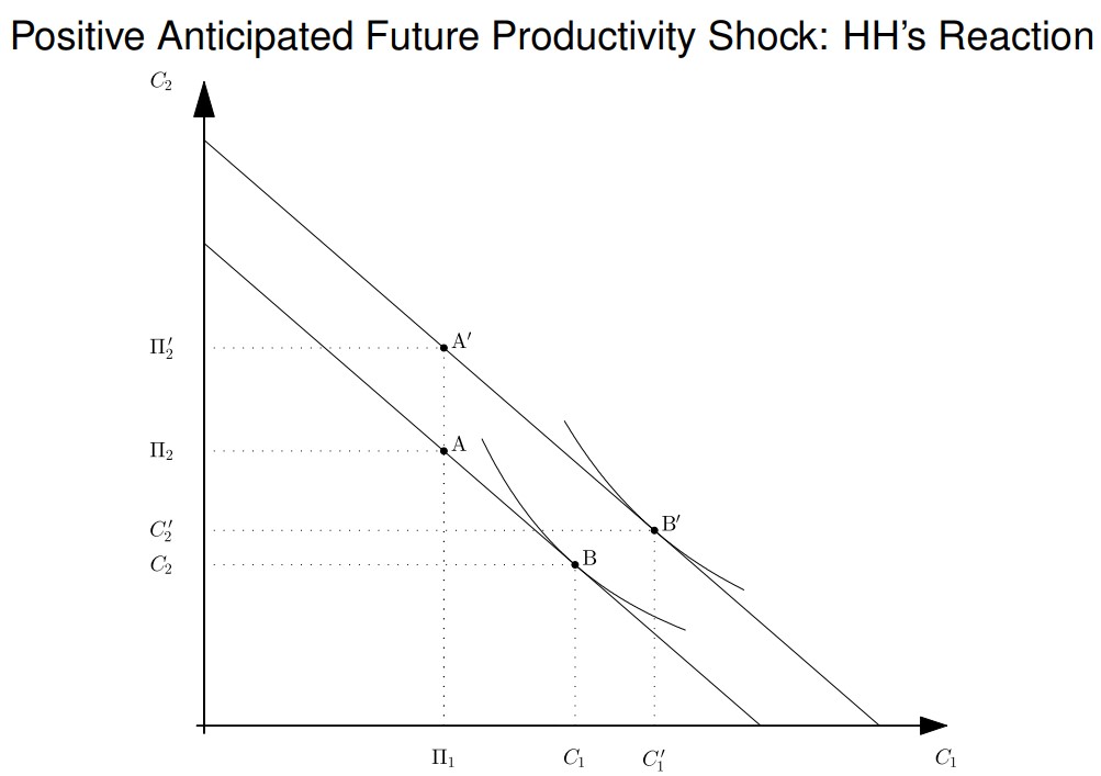
Summary

Assuming that $C_{1}$ is a normal good:

• Δ optimal investment: $A_{2}\uparrow\to I_{1}\uparrow$
• HH's reaction: $A_{2}\uparrow\to\Pi_{2}\uparrow\to S_{1}\downarrow$
• CA deteriorates: $\Delta CA_{1}\lt 0\,(CA_{1}=S_{1}-I_{1})$

Other Productivity Shocks

Other productivity shocks includes:

• negative anticipated future productivity shocks
• temporary productivity shocks $(A_{1}^{\prime}\neq A_{1},\,A_{2}^{\prime}=A_{2})$
• permanent productivity shocks $(A_{1}^{\prime}\gt A_{1},\,A_{2}^{\prime}\gt A_{2})$ or $(A_{1}^{\prime}\lt A_{1},\,A_{2}^{\prime}\lt A_{2})$

The HH's reaction to such a shock depends on:

• shock is positive or negative
• shock is temporary or permanent
• shock is anticipated or not

L5.1 - Int. R. Shocks in a Production Economy

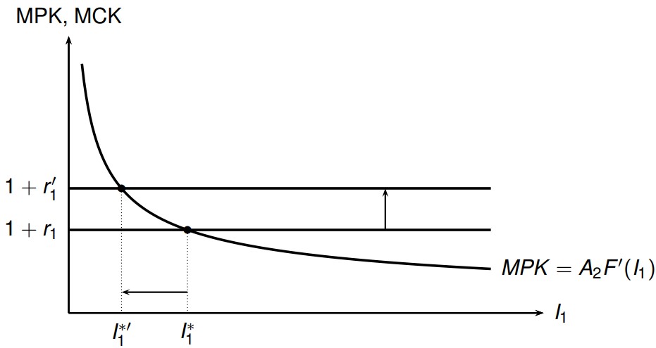
Firm's Reaction

A positive world interest rate shock:

• decreases the firm's investment level
• decreases output

Household's Reaction

If ${r}^{\ast}$ ↑ then HH's savings ($=\Pi_{2}-C_{1}$) increase

• Substitution effect (SE)
  • Saving in period 1 becomes more attractive
• Income effect (IE)
  • ${r}^{\ast}$ ↑ makes debtors poorer and creditors richer
• Additional income effect (IE2)
  • $\Pi_{2}$ (= area between MPK & MCK curves) decreases
• Assume $B_{0}^{h}=0$ and that $C_{1}$ and $C_{2}$ are normal goods

Overall, if the interest rate increases:

• SE < 0
• IE2 < 0 (as $C_{1}$ is normal)
• If the country is a debtor ($\Pi_{1}\lt C_{1}^{A}$):
  • IE < 0 as budget line shift that determines IE is to the left
  • TE = SE + IE + IE2 < 0
• If the country is a creditor ($\Pi_{1}\gt C_{1}^{A}$):
  • IE > 0 as budget line shift that determines IE is to the right
  • TE > or < 0 depending on which of SE + IE2 and IE dominates
  • Economists usually consider that TE < 0

Adjustment to a World Interest Shock

Collateral Constraints and Financial Shocks

So far, we assumed that the firm can borrow freely in period 1.

In reality, firms cannot borrow freely (financial frictions)

• e.g. Firms may not be able to commit to repay

We assume that the firm can borrow up to a collateral constraint ($D_{1}^{f}\leq\kappa$)

• This constraint may or may not bind

firm's new optimal investment in period 1:

• constraint binds: $I_{1}=\kappa$
• constraint doesn't bind: $I_{1}^{nc}$ such that $A_{2}F^{\prime}(I_{1}^{nc})=(1+r_{1})$
• Therefore: $I_{1}=min\{\kappa,I_{1}^{nc}\}$

Shocks to $\kappa$ (financial shocks) yield interesting dynamics

L5.2 - Fiscal Deficits and CA Imbalances

Ricardian Equivalence: If government expenditures don't change, changes in the tax schedule and bond issuance don't affect the HH's consumption

Rules:

• Two-period small open economy: periods 1 and 2
• The single consumption good is perishable
• Traded in the financial market are private and government bonds (both measured in units of the consumption good)
• There is a representative household (HH) in the economy endowed with
  • $B_{0}^{h}$ units of the bond at the beginning of period 1
  • $Q_{1}$ units of the good in period 1
  • $Q_{2}$ units of the good in period 2
• There is a government
  • government has expenditures
  • government finances them by:
    • taxes
    • issuing debt
  • Government expenditures (exogeneous)
    • $G_{1}$ in period 1
    • $G_{2}$ in period 2
  • Taxes are levied as lump-sum taxes
    • $T_{1}$ in period 1
    • $T_{2}$ in period 2
  • Government assets (or debts if negative):
    • $B_{0}^{g}$: exogeneously given at beginning of Period 1
    • $B_{1}^{g}$: amount of government assets at the end of period 1
    • $B_{t}^{g}\lt 0$: public debt outstanding
• Interest Rates:
  • $r_{0}$ for the initial bond holdings
  • $r_{1}$ for bonds held at the end of period 1

Government's Budget Constraint

The government's budget constraints are:

• $G_{1}+B_{1}^{g}=(1+r_{0})B_{0}^{g}+T_{1}$
• $G_{2}+B_{2}^{g}=(1+r_{1})B_{1}^{g}+T_{2}$
• Where G = Expenditure; T = Tax Revenue

Assume transversality condition: $B_{2}^{g}=0$

Intertemporal government budget constraint

$G_{1}+\frac{G_{2}}{1+r_{1}}=(1+{r}_{0})B_{0}^{g}+T_{1}+\frac{T_{2}}{1+{r}_{1}}$

Household's Budget Constraint

The household's budget constraints are:

• $C_{1}+T_{1}+B_{1}^{h}=(1+r_{0})B_{0}^{h}+Q_{1}$
• $C_{2}+T_{2}+B_{2}^{h}=(1+r_{1})B_{1}^{h}+Q_{2}$

Assume transversality condition: $B_{2}^{h}=0$

HH's intertemporal budget constraint

$C_{1}+\frac{C_{2}}{1+r_{1}}=(1+r_{0})B_{0}^{h}+Q_{1}-T_{1}+\frac{Q_{2}-T_{2}}{1+r_{1}}$

Intertemporal Resource Constraint

NIIP Position: $B_{0}=B_{0}^{h}+B_{0}^{g}$ (at beginning of Period 1)

• $B_{0}$: Country's NIIP
• $B_{0}^{h}$: Private Net Assets
• $B_{0}^{g}$: Government Net Assets

Combine Gov and HH's Budget Constraint:

Steps

$C_{1}+G_{1}+\frac{C_{2}+G_{2}}{1+r_{1}}=(1+r_{0})(B_{0}^{g}+B_{0}^{h})+Q_{1}+(T_{1}-T_{1})+\frac{Q_{2}+(T_{2}-T_{2})}{1+r_{1}}$

$C_{1}+\frac{C_{2}}{1+r_{1}}=(1+r_{0})B_{0}+Q_{1}+\frac{Q_{2}}{1+r_{1}}-G_{1}-\frac{G_{2}}{1+r_{1}}$

$C_{1}+\frac{C_{2}}{1+r_{1}}=(1+r_{0})B_{0}+Q_{1}-G_{1}+\frac{Q_{2}-G_{2}}{1+r_{1}}$

Equilibrium

• Feasibility of the intertemporal allocation
  • $C_{1}+\frac{C_{2}}{1+r_{1}}=(1+r_{0})B_{0}+Q_{1}-G_{1}+\frac{Q_{2}-G_{2}}{1+r_{1}}$
• Optimality of the intertemporal allocation
  • $U_{1}(C_{1},C_{2})=(1+r_{1})U_{2}(C_{1},C_{2})$
• Interest rate parity condition
  • $r_{1}=r^{*}$

Logarithmic Utility Solution

$U(C_{1},C_{2})=\ln C_{1}+\ln C_{2}$

Steps

Note: Same with Lecture 3 Logarithmic Solution

Using derivatibe formula $\frac{d\ln(x)}{dx}=\frac{1}{x}$, we get:

$U_{1}(C_{1},C_{2})=\frac{\partial U(C_{1},C_{2})}{\partial C_{1}}=\frac{\partial(\ln C_{1}+\ln C_{2})}{\partial C_{1}}=\frac{1}{C_{1}}$

$U_{2}(C_{1},C_{2})=\frac{\partial U(C_{1},C_{2})}{\partial C_{2}}=\frac{\partial(\ln C_{1}+\ln C_{2})}{\partial C_{2}}=\frac{1}{C_{2}}$

Therefore, the equilibrium condition $U_{1}(C_{1},C_{2})=(1+r_{1})U_{2}(C_{1},C_{2})$ becomes ${\frac{1}{C_{1}}}=(1+r_{1}){\frac{1}{C_{2}}}$

From the above, we can derive $C_{2}=(1+r_{1})C_{1}$

By substituting into Feasibility of the intertemporal allocation, we get:

$C_{1}={\frac{1}{2}}[(1+r_{0})B_{0}+Q_{1}-G_{1}+{\frac{Q_{2}-G_{2}}{1+r_{1}}}]$

$C_{2}={\frac{1}{2}(1+r_{1})}[(1+r_{0})B_{0}+Q_{1}-G_{1}+{\frac{Q_{2}-G_{2}}{1+r_{1}}}]$

Note that:

• government expenditures show up
• taxes do not show up

From the above $C_{1}$ and $C_{2}$ (optimal consumption path):

• Changes in $G_{1}$ and $G_{2}$ affect the HH's consumption
• The following changes don't affect the consumption (as long as they satisfy intertemporal government budget constraint)
  • $T_{1}$ and $T_{2}$ (tax schedule)
  • $B_{1}^{g}$ (government's asset/debt position)

Ricardian Equivalence

Ricardian Equivalence: Even if the government decreases $T_{1}$ and $B_{1}^{g}$, and instead increases $T_{2}$ such that intertemporal government budget constraint remains satisfied, this won't affect the optimal consumption path

The Ricardian equivalence holds because the HH reacts to tax changes by adjusting its savings.

Consider a change $\Delta T_{1}$ in the period 1 tax $T_{1}$

Private Saving: $S_{1}^{p}={Q}_{1}+r_{0}B_{0}^{h}-T_{1}-C_{1}$

• Disposable Income: ${Q}_{1}+r_{0}B_{0}^{h}-T_{1}$
• Consumption: $C_{1}$

Since other variables in private saving don't change, we have: $\Delta S_{1}^{p}=-\Delta T_{1}$

Government saving: $S_{1}^{g}=r_{0}B_{0}^{g}+T_{1}-G_{1}$

• Revenues: $r_{0}B_{0}^{g}+T_{1}$
• Expenditure: $G_{1}$

Since other variables in government saving don't change, we have: $\Delta S_{1}^{g}=\Delta T_{1}$

National Saving $S_{1}=S_{1}^{p}+S_{1}^{g}$ doesn't change:

• $\Delta S_{1}=\Delta S_{1}^{p}+\Delta S_{1}^{g}=-\Delta T_{1}+\Delta T_{1}=0$

Current Account also doesn't change:

• $\Delta CA=\Delta S_{1}-\Delta I_{1}=0$
• $\Delta I_{1}=0$ because we did not model production
• SUW Ch. 8: model with production in which still $\Delta I_{1}=0$

Conclusion:

• The Ricardian equivalence holds because changes in private and government saving exactly offsets each other
• When the government changes the timing of taxes, rational households adjust their savings so that their consumption paths remain unaffected
• As a result, the CA balance also does not change

Twin Deficits in the U.S

Twin Deficits: both fiscal and current account deficits

Ronald Reagan (U.S. President, 1981 - 1989)

• Implemented tax cuts
• Increased military spending

As a result, the fiscal deficit increased by roughly 3% of GDP

The Ricardian equivalence says:

• Changes in taxes $(T_{1},T_{2})$ do not affect the CA
• Changes in $(G_{1},G_{2})$ can affect the CA balance
  • However, the government spending increased only by 1.5% of GNP

If the Ricardian equivalence fails, a change in tax schedule can affect consumption choices.

Intergenerational effects: Those who benefit from the tax cut (today's generations) may not be the ones that pay for the future tax increase (future generations)

• to obtain quantitatively plausible effect, all HHs have to die after one period

Distortionary taxes: changes in tax rates will tend to distort consumption, savings, and investment decisions

• We have assumed taxes are lump-sum taxes
• In reality, taxes are specified as a fraction of consumption, income, firm's profits, etc.

Therefore, the explanation likely has to rely on a combination of:

• an increase in governement expenditures
• factors that break the Ricardian equivalence:
  • Borrowing constraints
  • Intergenerational effects
  • Distortionary taxes

L6 - Uncertainty and the CA

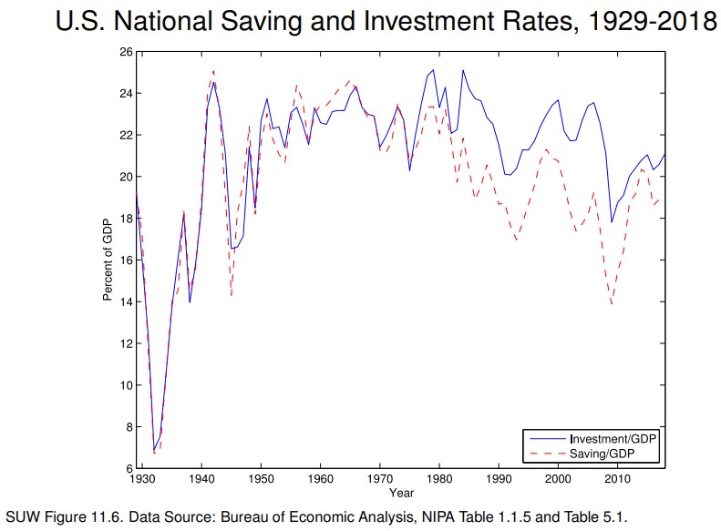
The Great Moderation in the U.S.

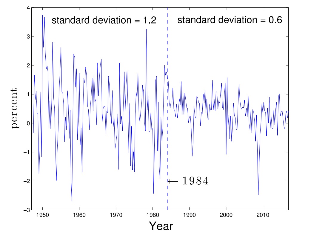
The Great Moderation: The volatility of the growth rate of real U.S. GDP per capita declined significantly after (about) 1984.

Three proposed explanations:

• Good-luck hypothesis: by chance, the U.S. economy has been blessed with smaller shocks.
• Good-policy hypothesis: volatility declined due to
  • good monetary policy (aggressive low inflation policy of Volcker and Greenspan Feds)
  • the phasing out of Regulation Q's interest rate ceilings for most types of bank deposits (such ceilings may cause negative real interest rates on deposits if inflation is high, causing bank deposits withdrawals, consequently reduced bank loans, and finally a credit-crunch-induced recession)
• Structural change hypothesis: the amplitude of business cycles was reduced by structural change, particularly in inventory management and in the financial sector

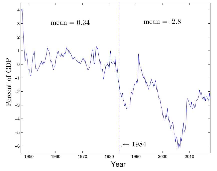
U.S. CA-to-GDP Ratio, 1947Q1 - 2017Q4

• 1947-1983: on average, CA surplus of 0.34% of GDP
• 1984-2017: on average, CA deficit of 2.8% of GDP

Open Economy Model with Uncertainty

Implication for CA

• High uncertainty about the future ($\sigma$ large)
  • People save more; The CA improves
• Low uncertainty about the future ($\sigma$ small; Great Moderation)
  • People save less; The CA deteriorates

Rules:

• Two-period small open economy: periods 1 and 2
• The single consumption good is perishable
• The single asset traded in the financial market is a bond (measured in units of the consumption good)
• There is a representative household (HH) endowed with
  • $B_{0}$ = 0 units of the bond at the beginning of period 1
  • units of the good
    • period 1: $Q_{1}=Q$ units of the goods
    • period 2:
      • Good state (50%): $Q_{2}=Q+\sigma$
      • Bad state (50%): $Q_{2}=Q-\sigma$
      • Assume $\sigma\geq 0$
      • If $\sigma\gt 0$ then period 2 is uncertain
• Interest Rates:
  • $r_{0}$ for the initial bond holdings,
  • $r_{1}=0$ for the bonds held at the end of period 1

Expected Utility Assumption

The HH cares about expected utility from consumption: $U(C_{1},C_{2}(\cdot))=\ln C_{1}+E\,[\ln C_{2}]$

With good state (G) and a bad state (B): $U(C_{1},C_{2}(\cdot))=\ln C_{1}+[\pi_{G}\ln C_{2}(G)+\pi_{B}\ln C_{2}(B)]$

• $\pi_{G}$: probability of the good state
• $\pi_{B}$: probability of the bad state
• $C_{2}(G)$: consumption in the good state
• $C_{2}(B)$: consumption in the bad state

Since we assume $\pi_{G}=\pi_{B}=\frac{1}{2}$, we have:

$U(C_{1},C_{2}(\cdot))=\ln C_{1}+[\frac{1}{2}\ln C_{2}(G)+\frac{1}{2}\ln C_{2}(B)]$

Household's Budget Constraint

The HH's budget constraints are:

• $C_{1}+B_{1}=(1+r_{0})\cdot0+Q$ ($B_{1}=Q-C_{1}$)
• $C_{2}(G)=(1+0)\cdot B_{1}+Q+\sigma$ ($C_{2}(G)=2Q+\sigma-C_{1}$)
• $C_{2}(B)=(1+0)\cdot B_{1}+Q-\sigma$ ($C_{2}(B)=2Q-\sigma-C_{1}$)

The household's utility maximization problem is:

$\max_{C_{1},C_{2}(G),C_{2}(B)}(\ln\,C_{1}+[{\frac{1}{2}}\ln\,C_{2}(G)+{\frac{1}{2}}\ln\,C_{2}(B)])$

Substituting $C_{2}(G)$ and $C_{2}(B)$, we obtain:

$\max_{C_{1}}(\ln C_{1}+[{\frac{1}{2}}\ln(2Q+\sigma-C_{1})+{\frac{1}{2}}\ln(2Q-\sigma-C_{1})])$

Therefore, the household picks $C_{1}$ to maximize her expected utility.

Maximization Condition: If $f^{\prime}(x^{*})=0$ and $f^{\prime\prime}(x)\lt 0$ (strictly concave), then $x^{*}$ is a global maximum of $f$

Let $f(C_{1})=(\ln C_{1}+[{\frac{1}{2}}\ln(2Q+\sigma-C_{1})+{\frac{1}{2}}\ln(2Q-\sigma-C_{1})])$

2nd_derivative

Note: Use Chain Rule

$f^{\prime}(C_{1})=\frac{1}{C_{1}}+\frac{1}{2}\cdot\frac{(-1)}{2Q+\sigma-C_{1}}+\frac{1}{2}\cdot\frac{(-1)}{2Q-\sigma-C_{1}}$

$f^{\prime}(C_{1})=(C_{1})^{-1}-\frac{1}{2}\cdot(2Q+\sigma-C_{1})^{-1}-\frac{1}{2}\cdot(2Q-\sigma-C_{1})^{-1}$

$f^{\prime\prime}(C_{1})=(-1)(C_{1})^{-2}-\frac{1}{2}(-1)(2Q+\sigma-C_{1})^{-2}(-1)-\frac{1}{2}(-1)(2Q-\sigma-C_{1})^{-2}(-1)$

$f^{\prime\prime}(C_{1})=-(C_{1})^{-2}-\frac{1}{2}(2Q+\sigma-C_{1})^{-2}-\frac{1}{2}(2Q-\sigma-C_{1})^{-2}$

We can clearly see that all terms are negative

$f^{\prime\prime}(C_{1})\lt 0$ ($f^{\prime}(C_{1})=0$ maximizes the HH's expected utility)

Let $f^{\prime}(C_{1})=0$, we have:

$\frac{1}{C_{1}}-\frac{1}{2}[\frac{1}{2Q+\sigma-C_{1}}+\frac{1}{2Q-\sigma-C_{1}}]=0$

Or $\frac{1}{C_{1}}=\frac{1}{2}[\frac{1}{2Q+\sigma-C_{1}}+\frac{1}{2Q-\sigma-C_{1}}]$

Case w/o Uncertainty

Without Uncertainty: $\sigma=0$

$\frac{1}{C_{1}}=\frac{1}{2}[\frac{1}{2Q-C_{1}}+\frac{1}{2Q-C_{1}}]$

steps

$\frac{1}{C_{1}}=\frac{1}{2Q-C_{1}}$

$C_{1}=2Q-C_{1}$

Thus $C_{1}=Q$

Therefore consumption in periods 1 and 2 is the same

• $C_{2}(G)=C_{2}(B)=2Q-C_{1}=Q$
• $TB_{1}=Q-C_{1}=0$
• $CA_{1}=r_{0}B_{0}+TB_{1}=TB_{1}=0$
• the HH does not need to save or borrow because the endowment stream is already perfectly smooth

Case with Uncertainty

From $\frac{1}{C_{1}}=\frac{1}{2}[\frac{1}{2Q+\sigma-C_{1}}+\frac{1}{2Q-\sigma-C_{1}}]$

steps

$\frac{1}{C_{1}}=\frac{1}{2}[\frac{4Q-2C_{1}}{(2Q-C_{1})^{2}-\sigma^{2}}]$

$4Q^{2}-4QC_{1}+C_{1}^{2}-\sigma^{2}=C_{1}(2Q-C_{1})$

$2C_{1}^{2}-6QC_{1}+4Q^{2}-\sigma^{2}=0$

$C_{1}=\frac{6Q\pm\sqrt{36Q^{2}-8(4Q^{2}-\sigma^{2})}}{4}$

We can obtain $C_{1}={\frac{3Q\pm{\sqrt{Q^{2}+2\sigma^{2}}}}{2}}$

However, $C_{1}={\frac{3Q+{\sqrt{Q^{2}+2\sigma^{2}}}}{2}}$ is not feasible

• $\frac{3Q+\sqrt{Q^{2}+2\sigma^{2}}}{2}\gt \frac{3Q+\sqrt{Q^{2}}}{2}=2Q$
• Recall that:
  • $C_{2}(G)=2Q+\sigma-C_{1}$
  • $C_{2}(B)=2Q-\sigma-C_{1}$
• If $C_{2}>0$, then $C_{1}\leq2Q-\sigma$

Therefore, the only solution is $C_{1}=\frac{3Q-{\sqrt{Q^{2}+2\sigma^{2}}}}{2}$

Finally we have:

• $C_{2}(G)=2Q+\sigma-\frac{3Q-{\sqrt{Q^{2}+2\sigma^{2}}}}{2}$
• $C_{2}(B)=2Q-\sigma-\frac{3Q-{\sqrt{Q^{2}+2\sigma^{2}}}}{2}$

Analysis

$C_{1}={\frac{3Q-{\sqrt{Q^{2}+2\sigma^{2}}}}{2}}=Q-\frac{\sqrt{Q^{2}+2\sigma^{2}}-Q}{2}$

• precautionary saving: $\frac{\sqrt{Q^{2}+2\sigma^{2}}-Q}{2}$
• If $\sigma =0$, then precautionary savings are zero.
• $\sigma$ ↑ >> precautionary saving ↑ >> $C_{1}$ ↓

$C_{2}(B)=Q-\sigma +\frac{\sqrt{Q^{2}+2\sigma^{2}}-Q}{2}$

• $Q_{2}=Q-\sigma$
• When $\sigma$ increases, $Q_{2}$ decreases in the bad state
• The household tries to avoid low consumption in the bad state by increasing her precautionary saving
• This has an implication for the CA as well

Implication for CA

$TB_{1}=Q-C_{1}(\sigma)$

Since $CA_{1}=r_{0}B_{0}+TB_{1}$ and $B_{0}=0$ (assumption):

• $CA=TB_{1}=Q-C_{1}(\sigma)$
• In response to an increase in uncertainty $\sigma$, the HH uses the trade balance as a vehicle to save in period 1

Therefore the conclusion:

• High uncertainty: People save more; The CA improves
• Low uncertainty: People save less; The CA deteriorates

L7 - External Adjustment in Open Economies

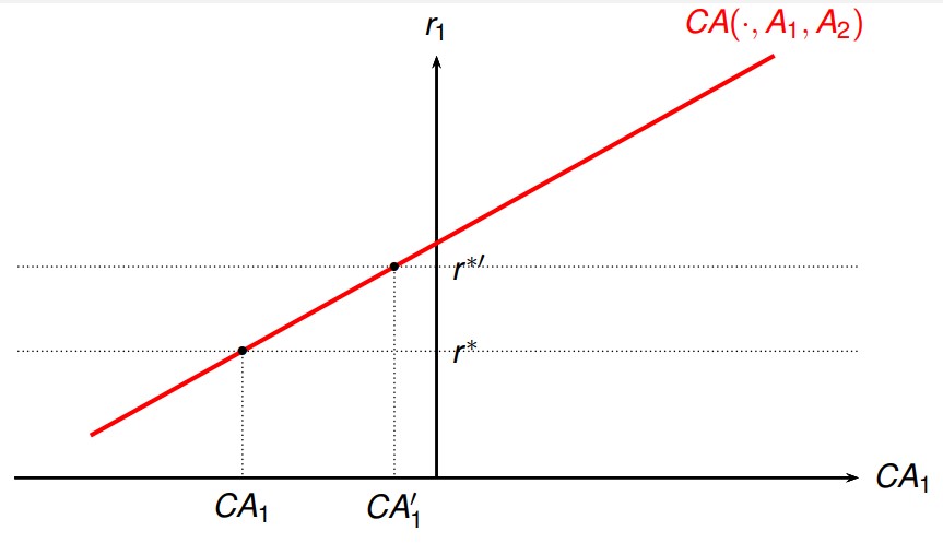
Current Account Schedule

The current account balance is an increasing function of $r_{1}$

Interest Rate Shock

• A positive shock to the interest rate ($r^{*}$ → $r^{*\prime}$)
• $CA_{1}$ improves if there is a positive interest rate shock

Temporary Productivity Shock

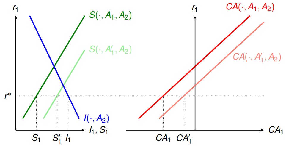
Following a positive shock to the period-1 efficiency parameter ($A_{1}$ → $A_{1}^{\prime}$), $CA_{1}$ improves

Anticipated Future Productivity Shock

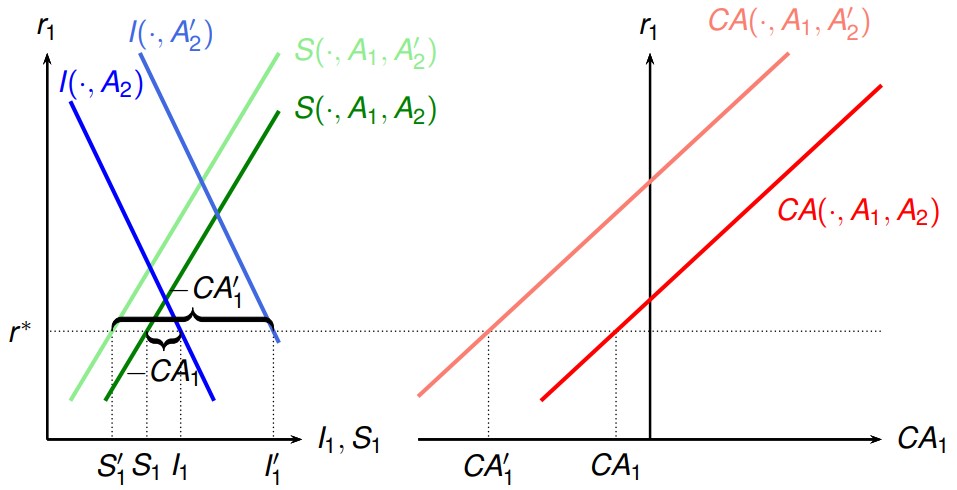
A positive shock to the period-2 efficiency parameter ($A_{2}$ → $A_{2}^{\prime}$), $CA_{1}$ deteriorates

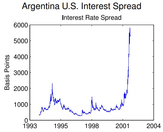
Country Risk Premium

• Emerging countries often face a higher interest rate
• when country is debtor, the world interest rate is raised by a country risk premium (p)
  • If $CA_{1}\geq0$, no risk premium
  • If $CA_{1}\lt0$, risk premium p
• accumulates more debt -> higher interest rate

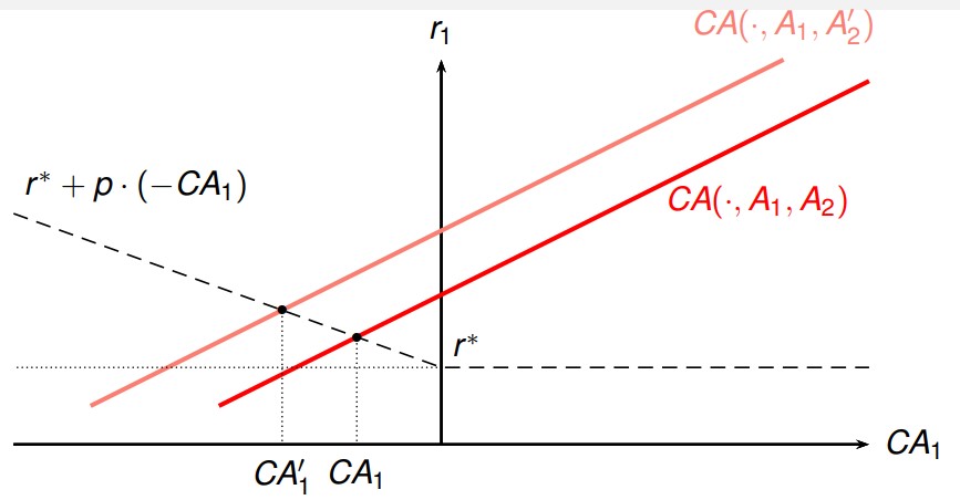
Positive anticipated future productivity shock: If $CA_{1}\lt0$, then an investment surge leads to a smaller CA deterioration than with a constant risk premium

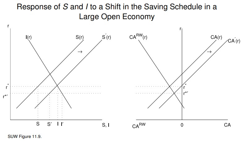
Large Open Economy

Two-country model:

• the U.S.
• the rest of the world (RW)

$CA^{US}=-CA^{RW}$

Important: Now, the U.S. CA balance affects the world interest rate.

Investment Surge in a Large Open Economy

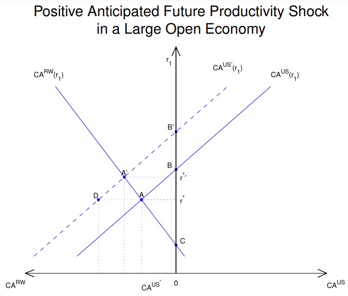
• Following the positive anticipated future productivity shock in the U.S. economy:
  • The U.S. CA schedule shifts left from $CA^{US}$ to $CA^{US\prime}$
  • The equilibrium point moves from A to $A^{\prime}$
• The resulting change in the U.S.:
  • CA is smaller
  • domestic interest rate is larger than the one in a small open economy setup
  • In a small open economy, the eqm. moves from A to D
• The resulting change in the U.S.:
  • CA is larger
  • domestic interest rate is smaller than the one in a closed economy setup
  • In a closed economy $CA = 0$ and the equilibrium moves from B to $B^{\prime}$

The U.S. Current Account Deficit

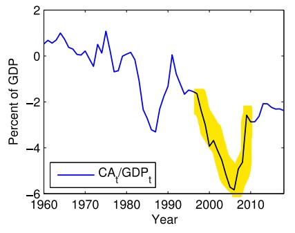
CA deficit: during 1996-2006 ballooned from 1.5% to 6% of GDP, then sharply improved to ≤ 3% of GDP by 2009. Is it driven by domestic or external factors?

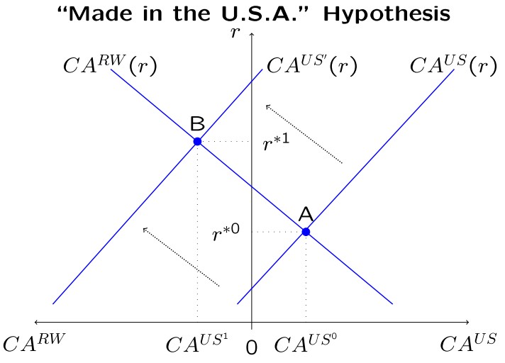
Made in the U.S.A. hypothesis

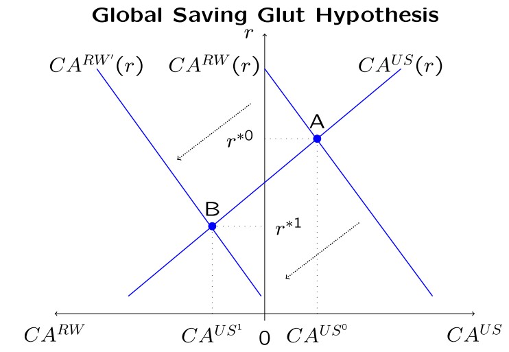
Global Saving Glut hypothesis

Test the hypothesis

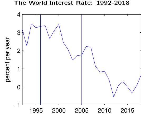
Period of 1996-2005 (global saving glut hypothesis)

• The world interest rate fell during this period

Period of 2006-2018 (made in the U.S.A. hypothesis)

• The CA deficit actually improved during this period
• Under the global saving glut hypothesis, this would be attributed to a decline in saving in the rest of the world and be accompanied by an increase in the world interest rate
• However, the world interest rate fell during 2005-2018

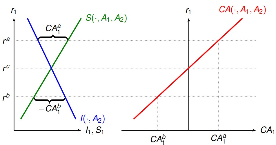
Large Open Economies Analysis

Key: Both countries affect the world interest rate

Setup:

• Two periods: periods 1 and 2
• Two countries: China (C) and the United States (US)
• The single consumption good is perishable
• The single asset traded in the financial markets is a bond (measured in units of the consumption good)
• In each country $x \in \{C, US\}$, there is a representative household (HH) endowed with
  • $B^x_0 = 0$ units of the bond at the beginning of period 1
  • $Q^x_1$ units of the good in period 1
  • $Q^x_2$ units of the good in period 2
• Interest Rates for bonds held at the end of period 1:
  • $r_1$ for the U.S
  • $r^C_1$ for China
  • $r^*_1$ for the world

An equilibrium requires six conditions:

• Feasibility and optimality in China
  • $C_1^C + \frac{C_2^C}{1+r_1^C} = Q_1^C + \frac{Q_2^C}{1+r_1^C}$
  • $U_1(C_1^C, C_2^C) = (1 + r_1^C)U_2(C_1^C, C_2^C)$
• Feasibility and optimality in the U.S.
  • $C_1^{US} + \frac{C_2^{US}}{1+r_1} = Q_1^{US} + \frac{Q_2^{US}}{1+r_1}$
  • $U_1(C_1^{US}, C_2^{US}) = (1 + r_1)U_2(C_1^{US}, C_2^{US})$
• Interest rate and current account conditions
  • $r_1 = r_1^C = r_1^*$
  • $CA^C(r^*) + CA_1^{US}(r^*) = 0$

Assume log utility for both countries: $U(C_1, C_2) = \ln C_1 + \ln C_2$

We have:

• $C_1^C = \frac{1}{2} (Q_1^C + \frac{Q_2^C}{1 + r_1^C})$
• $C_2^C = \frac{1}{2} (1 + r_1^C)(Q_1^C + \frac{Q_2^C}{1 + r_1^C})$
• $C_1^{US} = \frac{1}{2}[Q_1^{US} + \frac{Q_2^{US}}{1 + r_1}]$
• $C_2^{US} = \frac{1}{2} (1 + r_1)[Q_1^{US} + \frac{Q_2^{US}}{1 + r_1}]$

Assume China's endowment is growing:

• Let $Q$ denote some specific amount of the good
• $Q_1^C = \frac{1}{2} Q$ and $Q_2^C = Q$
• $Q_1^{US} = Q$ and $Q_2^{US} = Q$

In this case, we can show that:

• $C_1^C = \frac{1}{2}[\frac{1}{2} Q + \frac{Q}{1 + r_1^C}]$
• $C_2^C = \frac{1}{2} (1 + r_1^C)[\frac{1}{2} Q + \frac{Q}{1 + r_1^C}]$
• $C_1^{US} = \frac{1}{2}[Q + \frac{Q}{1 + r_1}]$
• $C_2^{US} = \frac{1}{2} (1 + r_1)[Q + \frac{Q}{1 + r_1}]$

This implies:

• $CA_1^C = TB_1^C + rB_0^C = TB_1^C = Q_1^C - C_1^C = \frac{1}{4}Q\frac{r_{1}^{C}-1}{1+r_{1}^{C}}$ (1)
• $CA_1^{US} = TB_1^{US} + rB_0^{US} = TB_1^{US} = Q_1^{US} - C_1^{US} = \frac{1}{2}Q\frac{r_{1}}{1+r_{1}}$ (2)

Now we can solve for the world interest rate $r_1^*$ using:

• $r_1 = r_1^C = r_1^*$ (3)
• $CA_1^C(r^*) + CA_1^{US}(r^*) = 0$ (3)

In this example, (1)-(4) imply: $r_1^* = \frac{1}{3}$

To solve other variables:

• Once we calculated $r_1^*$, other variables are easily obtained
• Using $r_1 = r_1^C = r_1^*$, we can solve for $(C_1^C, C_2^C)$ and $(C_1^{US}, C_2^{US})$
• $CA_1^C$ and $CA_1^{US}$ can be calculated from (1)-(2)
• $(TB_1^C, TB_2^C)$, $(TB_1^{US}, TB_2^{US})$, $B_1^C$ and $B_1^{US}$ can be also calculated

Capital Control in a Large Open Economy

• In this example:
  • China is a debtor in the first period $B_1^C = CA_1^C < 0$
  • the U.S. is a creditor in the first period
• Because China is a debtor, if it can lower the world interest rate, it would improve China's domestic welfare
• Therefore, China has an incentive to improve its CA balance in order to drive down the world interest rate
• The Chinese government may want to try to influence the world interest rate through capital control
  • E.g., it may try to induce the Chinese HH to consume less and save more in period 1
  • To this end, it may impose a “capital control tax” on international borrowing to increase the domestic interest rate

L8 - PPP and the Real Exchange Rate

The real exchange rate measures how expensive a foreign
country is relative to the home country. It measures the price of a basket of goods abroad in terms of baskets of good at home.

Law of One Price (LOOP)

The Law of One Price for a particular good holds if $P = \varepsilon P^*$.

Here:

• $P$ = good's domestic-currency price in the domestic country
• $P^*$ = good's foreign-currency price in the foreign country
• $\varepsilon$ = nominal exchange rate
  • $\varepsilon$ is the domestic-currency price of one unit of foreign currency
  • $\varepsilon$ (or $\frac{1}{\varepsilon}$) is what TV news report as an exchange rate
• E.g.: If 1kg of apples costs 7.33USD in the U.S., $\varepsilon$ = 1.5 & LOOP holds, then 1kg of apples costs 11AUD in Australia

However, the real world is not frictionless!

• LOOP hold well:
  • commodities: gold, oil, soy beans, wheat
  • luxury consumer goods: Rolex watches
• LOOP not hold well:
  • personal services: health care, education, restaurant meals, haircuts
  • housing, utilities
  • transportation

Big Mac index

The idea is to compare

• the price of a Big Mac in a foreign country: $P_{BigMac}^*$
• the price of a Big Mac in the U.S.: $P_{BigMac}$
• To compare these prices, define the Big Mac index by $e^{BigMac} = \frac{\varepsilon P^{BigMac*}}{P^{BigMac}}$
• The LOOP for BigMacs holds if and only if $e^{BigMac} = 1$

The Big-Mac Real Exchange Rate, January 2019

Country	$P^{BigMac*}$	$\varepsilon$	$\varepsilon P^{BigMac*}$	$e^{BigMac}$	$e^{BigMac PPP}$
Switzerland	6.50	1.02	6.62	1.19	0.86
United States	5.58	1	5.58	1	1
Canada	6.77	0.75	5.08	0.91	0.82
Euro area	4.05	1.15	4.64	0.83	1.38
China	20.90	0.15	3.05	0.55	0.27
India	178	0.01	2.55	0.46	0.03
Russia	110.17	0.01	1.65	0.30	0.05

Conclusion:

• For the Big Mac, the Law of One Price clearly fails
• The last column shows the PPP exchange rate for Big Macs, $e^{BigMac PPP} = \frac{P^{BigMacUS}}{P^{BigMac*}}$

Purchasing Power Parity (PPP)

Purchasing power parity (PPP) is a generalization of the
law of one price

The real exchange rate is defined as $e = \frac{\varepsilon P^*}{P}$

• $P$ = domestic currency price of a (representative) domestic basket of goods
• $P^*$ = foreign price of a (representative) foreign basket of goods
• $\varepsilon$ = nominal exchange rate

We say (absolute) PPP holds when $e = 1$ or $P = \varepsilon P^*$.

Relative PPP

We say that relative PPP holds when $\Delta e = 0$.

• $P$ = domestic consumer price index
• $P^*$ = foreign consumer price index
• $e = \frac{\varepsilon P^*}{P}$

Relative PPP can be tested with CPI data

To understand what relative PPP implies, consider:

• $\varepsilon_{t+1} = \frac{\varepsilon_{t+1} P^*_{t+1}}{P_{t+1}}$
• $\varepsilon_t = \frac{\varepsilon_t P^*_t}{P_t}$

Let $\Delta x \equiv \frac{x_{t+1}}{x_t} - 1$. Then, by dividing $e_{t+1}$ by $e_t$, we get: $(1 + \Delta e) = \frac{(1 + \Delta \varepsilon)(1 + \Delta P^*)}{(1 + \Delta P)}$

Taking logarithms on both sides and recalling that $\ln(1 + x) \approx x$ for $x$ small, we get: $\Delta e \approx \Delta \varepsilon + \Delta P^* - \Delta P$

Finally, if relative PPP holds then $\Delta e = 0$ and $\Delta P = \Delta \varepsilon + \Delta P^*$

• Relative PPP restricts the joint evolution of $P$, $P^*$, and $\varepsilon$
• To test the above equation, we only need to know changes

PPP Summary

• Absolute PPP doesn't hold in the data
• Relative PPP holds in the long-run data
• Relative PPP doesn't hold in the short run data

Nontradable Goods

Possible reason for the failure of PPP: nontradable goods (haircut, restaurant meals, housing, some health services, some educational services, fresh lettuce, etc)

Setup:

• Tradable goods prices: $P_T$ and $P_T^*$
• Nontradable goods prices: $P_N$ and $P_N^*$
• Suppose the LOOP holds for tradable goods so that $P_T = \varepsilon P_T^*$
• Suppose the LOOP does not hold for nontradable goods so that $P_N \neq \varepsilon P_N^*$
• Assume that the aggregate price level is some average of $P_T$ and $P_N$ as given by $P = \phi(P_T, P_N)$
• The same for the foreign price level: $P^* = \phi(P_T^*, P_N^*)$
• We assume the following property for the function $\phi(\cdot, \cdot)$:
  • $\phi(P_T, P_N)$ is increasing in both $P_T$ and $P_N$
  • For every $\lambda > 0$, $\phi(\lambda P_T, \lambda P_N) = \lambda \phi(P_T, P_N)$

Then, we have $e = \frac{\varepsilon P^*}{P} = \frac{\varepsilon \phi(P_T^*, P_N^*)}{\phi(P_T, P_N)} = \frac{\varepsilon P_T^* \phi(1, P_N^* / P_T^*)}{P_T \phi(1, P_N / P_T)} = \frac{\phi(1, P_N^* / P_T^*)}{\phi(1, P_N / P_T)}$

• last equality holds because of LOOP ($P_T = \varepsilon P_T^*$)

Observe that in general, $e \neq 1$:

• $e \gtrless 1$ if and only if $\frac{P_N^*}{P_T^*} \gtrless \frac{P_N}{P_T}$
• With nontradable goods, absolute PPP systematically fails

Balassa-Samuelson Model

Think about two types of firms producing tradable and nontradable goods

• Production function for tradable goods: $Q_T = a_T L_T$
• Production function for nontradable goods: $Q_N = a_N L_N$
• Profit for the firm producing tradable goods: Profit = $P_T (a_T L_T)$ - $w L_T$
• Profit for the firm producing nontradable goods: Profit = $P_N (a_N L_N)$ - $w L_N$
• We assume free labor mobility and perfect competition in both output markets

Perfect competition implies zero profit for operating firms

• $P_T (a_T L_T)$ - $w L_T = 0$
• $P_N (a_N L_N)$ - $w L_N = 0$

These two equations imply:

• $P_{T}a_{T}=w$
• $P_{N}a_{N}=w$

Thus, we get: ${\frac{P_{T}}{P_{N}}}={\frac{a_{N}}{a_{T}}}$

Similarly, we can derive: $\frac{P_{T}^{*}}{P_{N}^{*}}=\frac{a_{N}^{*}}{a_{T}^{*}}$

By plugging in productivities, we get: $e = \frac{\phi(1, a_T^* / a_N^*)}{\phi(1, a_T / a_N)}$

If $\phi(P_{T},P_{N})\,=\,\sqrt{P_{T}P_{N}}$, we have $e = {\frac{\sqrt{a_{T}^{*}/a_{N}^{*}}}{\sqrt{a_{T}/a_{N}}}}$

The real exchange rate depends on the two countries' difference in relative productivities of tradables and nontradables

If $\frac{a_T}{a_N}$ increases over time then $e$ decreases:

• i.e., the real exchange rate appreciates (towards the domestic country)
• The domestic country becomes relatively more expensive

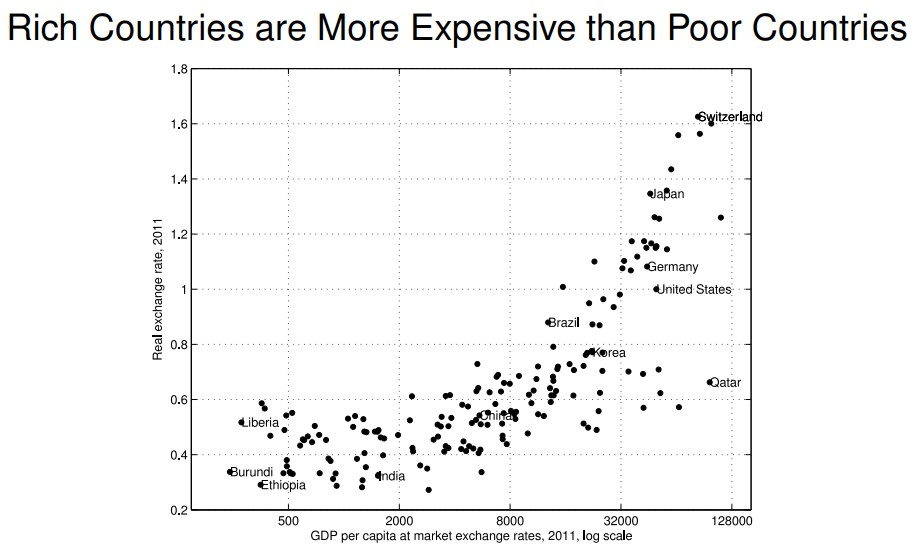
Countries with higher per capita GDP tend to be more expensive

In poor countries, the productivity for tradable goods $a_{T}^{*}$ is typically quite low.

For poor countries, we have: $e = \frac{\phi(1, a_T^* / a_N^*)}{\phi(1, a_T^{US} / a_N^{US})}$

Trade Barriers

Trade barriers (such as import tariffs, export subsidies, quotas) can also generate deviations from PPP

Consider a country with two types of (tradable) goods:

• Importable goods (the country imports some), with domestic price $P_M$ and world price $P_M^*$
• Exportable goods (the country exports some), with domestic price $P_X$ and world price $P_X^*$

First, if there are no trade barriers, the LOOP must hold for both types of goods:

• $P_M = \varepsilon P_M^*$
• $P_X = \varepsilon P_X^*$

Then, for the real exchange rate, we get:

$e = \frac{\varepsilon P^*}{P} = \frac{\varepsilon \phi(P_X^*, P_M^*)}{\phi(P_X, P_M)} = \frac{\phi(\varepsilon P_X^*, \varepsilon P_M^*)}{\phi(P_X, P_M)} = 1$

Without trade barriers, absolute PPP holds. The countries and the rest of the world are equally expensive.

Now with import tariff τ > 0, $P_M = (1+τ)\varepsilon P_M^*$, and we have:

$e = \frac{\varepsilon P^*}{P} = \frac{\varepsilon \phi(P_X^*, P_M^*)}{\phi(P_X, P_M)} = \frac{\phi(\varepsilon P_X^*, \varepsilon P_M^*)}{\phi(P_X, P_M)} = \frac{\phi(\varepsilon P_X^*, \varepsilon P_M^*)}{\phi(\varepsilon P_X^*, (1+τ)\varepsilon P_M^*)} < 1$

L9 - Sudden Stops and Real Exchange Rates

Sudden Stop: cutoff from international capital markets and hence capital inflows stopped abruptly

Sudden Stop Model

A sharp increase in the interest rate for borrowing, $r_1$ (harder to borrow from ROW)

Setup:

• 2 Periods
• Representative HH
• tradable and nontradable consumption goods
• There is a single asset, a bond, in this world (HH holds $B_0$ units at beginning)
• Endowment: The household is endowed with:
  • $Q_1^T$ units of tradables and $Q_1^N$ units of nontradables in period 1
  • $Q_2^T$ units of tradables and $Q_2^N$ units of nontradables in period 2
• Consumption: The household's consumption choices are
  • $C_1^T$ for tradables and $C_1^N$ for nontradables in period 1
  • $C_2^T$ for tradables and $C_2^N$ for nontradables in period 2
• Price of goods are determined in equilibrium:
  • $p_1$ = price of nontradables relative to that of tradables in period 1
  • $p_2$ = price of nontradables relative to that of tradables in period 2

Real Exchange Rate

The real exchange rate in each period (t = 1, 2) is defined as $e_t = \frac{\varepsilon_t P_t^*}{P_t}$

• $P_t \equiv \phi(P_t^T, P_t^N)$ is the aggregate price level for the home country
• $P_t^* \equiv \phi(P_t^{T*}, P_t^{N*})$ is the aggregate price level for the rest of the world

We assume that the function $\phi(\cdot, \cdot)$ has the following properties:

• $\phi(P_t^T, P_t^N)$ is increasing in both $P_T^t$ and $P_N^t$
• For every $\lambda > 0$, we have $\phi(\lambda P_T^t, \lambda P_N^t) = \lambda \phi(P_t^T, P_t^N)$

Then, we have $e_t = \frac{\varepsilon_t P_t^*}{P_t} = \frac{\varepsilon_t \phi(P_t^{T*}, P_t^{N*})}{\phi(P_t^T, P_t^N)} = \frac{\varepsilon_t P_T^{*t} \phi(1, P_t^{T*} / P_t^{N*})}{P_T^t \phi(1, P_t^T / P_t^N)} = \frac{\phi(1, P_t^{T*} / P_t^{N*})}{\phi(1, P_t^T / P_t^N)} = \frac{\phi(1, 1)}{\phi(1, p_t)}$

Here we assumed that the price ratio of nontradables and tradables in the ROW is constant; in particular: $\frac{P_t^{N*}}{P_t^{T*}} = 1$ for all $t = 1, 2$

Note also that we have, by definition, $\frac{P_t^N}{P_t^T} = p_t$ for all $t = 1, 2$

Household's Budget Constraint

The budget constraint is expressed in tradable goods as the unit of measure

Therefore, we have:

• $C_1^T + p_1 C_1^N + B_1 = (1 + r_0) B_0 + Q_1^T + p_1 Q_1^N$ (1)
• $C_2^T + p_2 C_2^N = (1 + r_1) B_1 + Q_2^T + p_2 Q_2^N$ (2)

By combining (1) and (2), we can derive the household's intertemporal budget constraint: $C_1^T + p_1 C_1^N + \frac{C_2^T + p_2 C_2^N}{1 + r_1} = (1 + r_0) B_0 + Q_1^T + p_1 Q_1^N + \frac{Q_2^T + p_2 Q_2^N}{1 + r_1}$

Utility Function with Tradables and Nontradables

$U(C_{1}^{T},C_{1}^{N},C_{2}^{T},C_{2}^{N})=ln C_{1}^{T}+ln C_{1}^{N}+ln C_{2}^{T}+ln C_{2}^{N}$

We extend to the four-good case:

• $-\frac{U_1}{U_2} = -\frac{1}{p_1}$
• $-\frac{U_1}{U_3} = -(1 + r_1)$
• $-\frac{U_1}{U_4} = -\frac{1}{p_2}(1 + r_1)$

And we have:

• $U_1 = \frac{\partial U(C_1^T, C_1^N, C_2^T, C_2^N)}{\partial C_1^T}$
• $U_2 = \frac{\partial U(C_1^T, C_1^N, C_2^T, C_2^N)}{\partial C_1^N}$
• $U_3 = \frac{\partial U(C_1^T, C_1^N, C_2^T, C_2^N)}{\partial C_2^T}$
• $U_4 = \frac{\partial U(C_1^T, C_1^N, C_2^T, C_2^N)}{\partial C_2^N}$

Resource Constraint

Market Clearing Conditions (all the nontradables are consumed within the country):

• $C_{1}^{N}=Q_{1}^{N}$
• $C_{2}^{N}=Q_{2}^{N}$

Therefore, $C_1^T + p_1 C_1^N + \frac{C_2^T + p_2 C_2^N}{1 + r_1} = (1 + r_0) B_0 + Q_1^T + p_1 Q_1^N + \frac{Q_2^T + p_2 Q_2^N}{1 + r_1}$ becomes the economy's resource constraint:

$C_1^T + \frac{C_2^T}{1 + r_1} = (1 + r_0) B_0 + Q_1^T + \frac{Q_2^T}{1 + r_1}$

Equilibrium

An equilibrium requires four conditions:

• Resource constraint
  • $C_1^T + \frac{C_2^T}{1 + r_1} = (1 + r_0) B_0 + Q_1^T + \frac{Q_2^T}{1 + r_1}$
• Optimality of the intertemporal allocation
  • $\frac{U_1}{1} = \frac{U_2}{p_1} = \frac{U_3}{\frac{1}{1 + r_1}} = \frac{U_4}{\frac{p_2}{(1 + r_1)}}$
• Interest rate parity condition
  • $r_1 = r^*$
• Market clearing for nontradable goods
  • $C_1^N = Q_1^N$
  • $C_2^N = Q_2^N$

Solve Equilibrium

Using the derivative formula, $\frac{d(\ln x)}{dx} = \frac{1}{x}$, we can get

• $U_1 = \frac{\partial (\ln C_1^T + \ln C_1^N + \ln C_2^T + \ln C_2^N)}{\partial C_1^T} = \frac{1}{C_1^T}$
• $U_2 = \frac{\partial (\ln C_1^T + \ln C_1^N + \ln C_2^T + \ln C_2^N)}{\partial C_1^N} = \frac{1}{C_1^N}$
• $U_3 = \frac{\partial (\ln C_1^T + \ln C_1^N + \ln C_2^T + \ln C_2^N)}{\partial C_2^T} = \frac{1}{C_2^T}$
• $U_4 = \frac{\partial (\ln C_1^T + \ln C_1^N + \ln C_2^T + \ln C_2^N)}{\partial C_2^N} = \frac{1}{C_2^N}$

Substitute the above to Optimality of the intertemporal allocation, we have:

• $-\frac{C_1^N}{C_1^T} = -\frac{1}{p_1}$ (3)
• $-\frac{C_2^T}{C_1^T} = -(1 + r_1)$ (4)
• $-\frac{C_2^N}{C_1^T} = -\frac{1}{p_2}(1 + r_1)$ (5)

From (4), we can obtain: $C_1^T = \frac{1}{2}[(1 + r_0)B_0 + Q_1^T + \frac{Q_2^T}{1 + r^*}]$

Then, we can subsequently derive:

• $C_2^T = \frac{1}{2}(1 + r^*)[(1 + r_0)B_0 + Q_1^T + \frac{Q_2^T}{1 + r^*}]$
• $C_1^N = Q_1^N$
• $C_2^N = Q_2^N$
• $p_1 = \frac{C_1^T}{Q_1^N}$
• $p_2 = \frac{C_2^T}{Q_2^N}(1 + r^*)$

A sudden stop involves:

• An improvement in the current account balance
• A real exchange rate depreciation
• A reduction in GDP

L10 - Sudden Stops and Unemployment

A Model of A Sudden Stop with Wage Rigidities

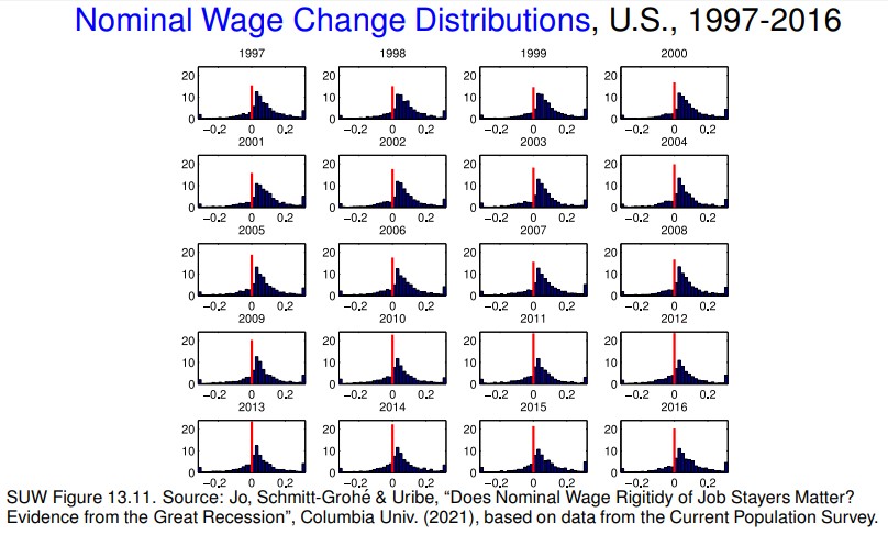
Nominal wage rigidities create unemployment after a sudden stop:

• a sudden stop generates a drop in the relative price of nontradables
• Since wages do not go down, firms reduce both employment and the production of nontradables

Setup:

• 2 Periods
• Representative HH and representative firm
  • the household owns the firm
  • The firm produces nontradables with labor input hired from the household
• tradable and nontradable consumption goods
• There is a single asset, a bond, in this world (HH holds $B_0$ units at beginning)
• Endowment: The household is endowed with:
  • $Q_1^T$ units of tradables and $Q_1^N$ units of nontradables in period 1
  • $Q_2^T$ units of tradables and $Q_2^N$ units of nontradables in period 2
• Consumption: The household's consumption choices are
  • $C_1^T$ for tradables and $C_1^N$ for nontradables in period 1
  • $C_2^T$ for tradables and $C_2^N$ for nontradables in period 2
• Labor endowment (which can be used in the production of nontradable goods):
  • The household is endowed with $\bar{h}$ units of labor in each period
  • $(h_1, h_2)$: The amounts of labor actually hired by the firm in periods 1 and 2
    • $h_t \leq \bar{h}$ for $t = 1, 2$
• Price of goods are determined in equilibrium:
  • $p_1$ = price of nontradables relative to that of tradables in period 1
  • $p_2$ = price of nontradables relative to that of tradables in period 2

Nominal Prices

• The prices $P_t^N$, $t = 1, 2$, of nontradables are determined in equilibrium by domestic demand and supply conditions
• The prices $P_t^T$, $t = 1, 2$, of tradables are determined by the LOOP ($P_t^T = \varepsilon_t P_t^{*}$)
  • nominal exchange rate $\varepsilon_t$ as an exogenously given policy decision
  • take $P_t^{*}$ as given (small economy)
  • assume $P_1^{*} = P_2^{*} = 1$ (for simplicity)
  • Therefore, $P_t^T = \varepsilon_t$ for $t = 1, 2$

The Firm's Problem

The firm owned by the household produces nontradable goods in this economy

• Labor input: $(h_1, h_2)$
• Wage per unit of labor: $(W_1, W_2)$
• Production technology: $Q_t^N = (h_t)^\alpha$ where $\alpha \in (0, 1)$

Firm's profit maximization problem in period $t = 1, 2$:

• $\max_{h_t \geq 0}[ P_t^N Q_t^N(h_t) - W_t h_t]$ (1)
  • $P_t^N Q_t^N(h_t)$: Revenues
  • $W_t h_t$: Labor Costs

Divide the profit function in problem (1) by $P_t^T$ to obtain

• $\max_{h_t \geq 0} \left[ \left( \frac{P_t^N}{P_t^T} \right) Q_t^N(h_t) - \left( \frac{W_t}{P_t^T} \right) h_t \right]$ (2)
  or
• $\max_{h_t \geq 0} [ p_t Q_t^N(h_t) - w_t h_t ]$,
  where
  • $p_t \equiv \frac{P_t^N}{P_t^T}$: price of nontradables relative to that of tradables
  • $w_t \equiv \frac{W_t}{P_t^T}$: real wage

Substituting in the production function we arrive at: $\max_{h_t \geq 0} [p_t (h_t)^\alpha - w_t h_t]$

$\Pi_t \equiv \max_{h_t \geq 0} [ p_t (h_t)^\alpha - w_t h_t ]$

• $p_t (h_t)^\alpha$: Revenues
• $w_t h_t$: Labor Costs

The firm's optimal choice of employment satisfies the FOC:

$MP = \frac{d (p_t (h_t)^\alpha)}{d h_t} = p_t \alpha (h_t)^{\alpha-1} = w_t = \frac{d (w_t h_t)}{d h_t} = MC$

The condition $p_t \alpha (h_t)^{\alpha-1} = w_t$ is also sufficient for profit maximization as:

• the production function $h_t^\alpha$ is strictly concave, and therefore
• the profit function $p_t h_t^\alpha - w_t h_t$ is strictly concave

Downward Nominal Wage Rigidities

If nominal wages are flexible, they adjust to achieve full employment. In that case, we have: $h_1 = h_2 = \bar{h}$

However, an important assumption of our model today are downward nominal wage rigidities

• Nominal wages do not adjust downwards in the short-run
• Thus the labor market may not clear. We can have $h_1 < \bar{h}$, $h_2 < \bar{h}$

Formally, taking $W_0$ as exogenously given, we assume:

• downward nominal wage rigidity $W_2 \geq W_1 \geq W_0$
• labor market slackness conditions $(W_2 - W_1)(\bar{h} - h_2) = (W_1 - W_0)(\bar{h} - h_1) = 0$

In fact, to simplify our analysis, we now assume that:

• $\varepsilon_1 = \varepsilon_2 = \bar{\varepsilon}$ (fixed exchange rate regime / currency peg)
• Nominal wages are rigid: $W_2 = W_1 = W_0$
• These assumptions imply that real wages are rigid: $\bar{w} \equiv w_1 = \frac{W_1}{P_1^T} = \frac{W_0}{\bar{\varepsilon}} = w_2 = \frac{W_2}{P_2^T} = \frac{W_0}{\bar{\varepsilon}}$

Household's Budget Constraints

The BCs are expressed in tradable goods as the unit of measure

Therefore, we have:

• $C_1^T + p_1 C_1^N + B_1 = (1 + r_0) B_0 + Q_1^T + w_1 h_1 + \Pi_1$ (3)
• $C_2^T + p_2 C_2^N = (1 + r_1) B_1 + Q_2^T + w_2 h_2 + \Pi_2$ (4)
• $h_t$ denotes the actual amount of labor employed by the firm in period $t$
• $w_1 h_1 + \Pi_1 = p_1 Q_1^N$
• $w_2 h_2 + \Pi_2 = p_2 Q_2^N$

(3) & (4) yield the intertemporal budget constraint:

$C_1^T + p_1 C_1^N + \frac{C_2^T + p_2 C_2^N}{1 + r_1} = (1 + r_0) B_0 + Q_1^T + p_1 Q_1^N + \frac{Q_2^T + p_2 Q_2^N}{1 + r_1}$

Resource Constraint

Market Clearing Conditions (all the nontradables are consumed within the country):

• $C_{1}^{N}=Q_{1}^{N}=(h_1)^\alpha$
• $C_{2}^{N}=Q_{2}^{N}=(h_2)^\alpha$

Therefore, $C_1^T + p_1 C_1^N + \frac{C_2^T + p_2 C_2^N}{1 + r_1} = (1 + r_0) B_0 + Q_1^T + p_1 Q_1^N + \frac{Q_2^T + p_2 Q_2^N}{1 + r_1}$ becomes the economy's resource constraint:

$C_1^T + \frac{C_2^T}{1 + r_1} = (1 + r_0) B_0 + Q_1^T + \frac{Q_2^T}{1 + r_1}$

Equilibrium

An equilibrium requires five conditions:

• Resource constraint
  • $C_1^T + \frac{C_2^T}{1 + r_1} = (1 + r_0) B_0 + Q_1^T + \frac{Q_2^T}{1 + r_1}$ (5)
• Optimality of the intertemporal allocation
  • $\frac{U_1}{1} = \frac{U_2}{p_1} = \frac{U_3}{\frac{1}{1 + r_1}} = \frac{U_4}{\frac{p_2}{(1 + r_1)}}$ (6)
• Interest rate parity condition
  • $r_1 = r^*$ (7)
• Market clearing for nontradable goods (8)
  • $C_{1}^{N}=Q_{1}^{N}=(h_1)^\alpha$
  • $C_{2}^{N}=Q_{2}^{N}=(h_2)^\alpha$
• Firm's optimization conditions (9)
  • $p_1 \alpha (h_1)^{\alpha-1} = \bar{w}$
  • $p_2 \alpha (h_2)^{\alpha-1} = \bar{w}$

Solve Equilibrium

Steps

Using the derivative formula, $\frac{d(\ln x)}{dx} = \frac{1}{x}$, we can get

• $U_1 = \frac{\partial (\ln C_1^T + \ln C_1^N + \ln C_2^T + \ln C_2^N)}{\partial C_1^T} = \frac{1}{C_1^T}$
• $U_2 = \frac{\partial (\ln C_1^T + \ln C_1^N + \ln C_2^T + \ln C_2^N)}{\partial C_1^N} = \frac{1}{C_1^N}$
• $U_3 = \frac{\partial (\ln C_1^T + \ln C_1^N + \ln C_2^T + \ln C_2^N)}{\partial C_2^T} = \frac{1}{C_2^T}$
• $U_4 = \frac{\partial (\ln C_1^T + \ln C_1^N + \ln C_2^T + \ln C_2^N)}{\partial C_2^N} = \frac{1}{C_2^N}$

Substitute the above to Optimality of the intertemporal allocation, we have:

• $-\frac{C_1^N}{C_1^T} = -\frac{1}{p_1}$ (10)
• $-\frac{C_2^T}{C_1^T} = -(1 + r_1)$ (11)
• $-\frac{C_2^N}{C_1^T} = -\frac{1}{p_2}(1 + r_1)$ (12)

From (11), we can obtain: $C_1^T = \frac{1}{2}[(1 + r_0)B_0 + Q_1^T + \frac{Q_2^T}{1 + r^*}]$

Then, we can subsequently derive:

• $C_1^T = \frac{1}{2}[(1 + r_0)B_0 + Q_1^T + \frac{Q_2^T}{1 + r^*}]$
• $C_2^T = (1 + r^*)C_1^T$
• $p_1 = \left( \frac{\bar{w}}{\alpha} \right)^\alpha (C_1^T)^{1-\alpha}$
• $p_2 = \left( \frac{\bar{w}}{\alpha} \right)^\alpha (C_2^T)^{1-\alpha}$
• $h_1 = \left( \frac{\alpha p_1}{\bar{w}} \right)^{\frac{1}{1-\alpha}}$
• $h_2 = \left( \frac{\alpha p_2}{\bar{w}} \right)^{\frac{1}{1-\alpha}}$
• $C_1^N = (h_1)^\alpha$
• $C_2^N = (h_2)^\alpha$

A sudden stop involves:

• An improvement in the current account balance
• An increase in the unemployment rate
• A moderate depreciation of the real exchange rate
  • The real exchange rate would depreciate more if nominal wages went down
• A reduction in GDP

L11 - International Capital Market Integration

Saving-Investment Correlations

Feldstein and Horioka (1980) document that national saving rates are highly correlated with investment rates

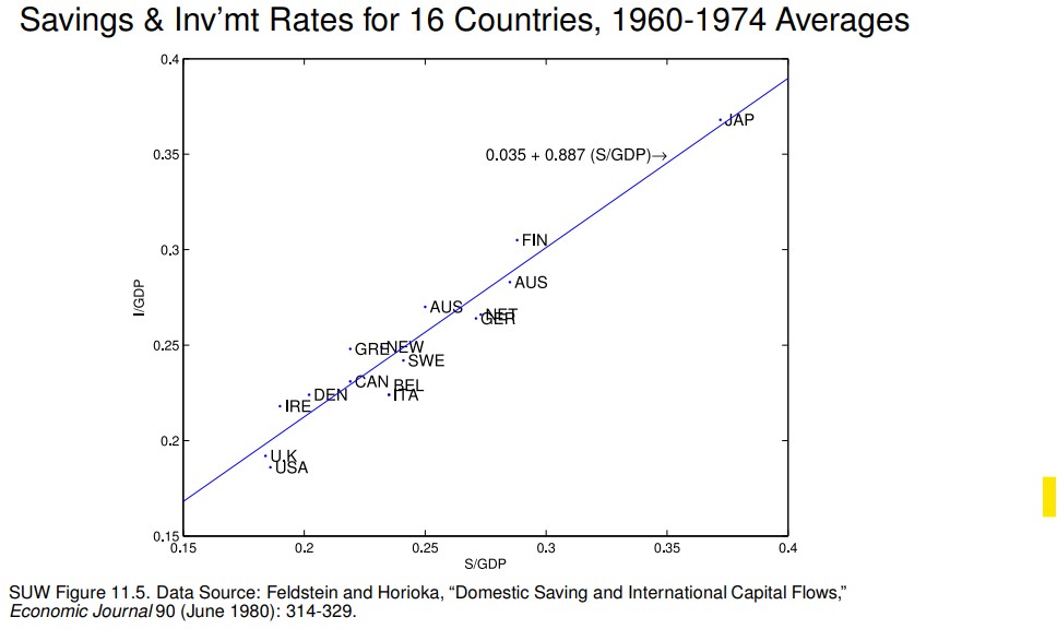
• 16 industrialized countries
• Data on average saving-to-GDP and investment-to-GDP rates during 1960-1974
• Cross-country OLS regression: $(\frac{I}{GDP})_i = \alpha + \beta (\frac{S}{GDP})_i + v_i$
  • $i$ indicates a country
  • $\alpha = 0.035$
  • $\beta = 0.887$ (strong positive correlation)
  • $R^2 = 0.91$ (91% of cross-country variation in $\frac{I}{GDP}$ explained by variations in $\frac{S}{GDP}$)

• Feldstein and Horioka (1980) argued:
  • If capital was highly mobile across countries, then the correlation between saving and investment should be ≈ 0
  • In their view, above empirical findings thus evidence low capital mobility
• To understand their position, recall that $CA(r) = S(r) - I(r)$
• degree of capital mobility - measuring the comovement of saving and investment

Feldstein and Horioka (1980)

In a closed economy, $S = I$

• Comovement of $S$ and $I$
• The lack of (cross-border) capital mobility -> high correlation between $S$ and $I$
• Regressing $\left( \frac{I}{GDP} \right)$ on $\left( \frac{S}{GDP} \right)$ -> $\beta$ is positive and significant if countries are closed

In an open economy, $S$ and $I$ do not have to move together

• We expect that $\beta$ is insignificant under free capital mobility

For the 16 industrialized countries (cross-country analysis):

• During the period 1960-1974, $\beta$ = 0.887
• For the later period 1974-1990, $\beta$ = 0.495

For the U.S. (time-series analysis):

• During the period 1955-1979, $\beta$ = 1.05
• For the later period 1980-1987, $\beta$ = 0.03

Feldstein and Horioka -> these results imply that the mobility of capital has increased over time

However: Observing high correlations between S and I need not be informative about the degree of international capital market integration

A high correlation between S and I doesn't necessarily imply that an economy is financially closed!

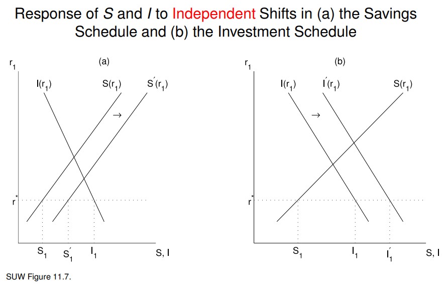
Counterexample 1: Same shock shifts both the saving and the investment schedule

• Small open production economy with perfect capital mobility
• $Q_t = A_tF(I_{t-1})$ for $t = 1, 2$
• Permanent positive productivity shock: $\Delta A_1 \gg \Delta A_2 > 0$
  • $A_2 \uparrow$: I shifts right
  • $A_2 \uparrow$: $\Pi_2 \uparrow$
  • $A_1 \uparrow$: $\Pi_1 \uparrow$
  • $\Delta A_1 \gg \Delta A_2$: plausible that $\Pi_1$ increases more than $\Pi_2$
  • Thus S shifts right as the consumption-smoothing HH saves more in period 1
• Despite free capital mobility, the shock generates a spurious comovement of saving and investment

Counterexample 2: Large country effects

• Large open economy with perfect capital mobility.
• Shock that shifts saving schedule to the right.
  • domestic CA schedule shifts to the right
  • $\to$ world interest rate falls
  • $\to$ domestic investment schedule shifts to the right.
• Despite free capital mobility, the shock generates a spurious comovement of saving and investment

The Covered Interest Rate Parity

An alternative way to measure capital mobility is to check the covered interest rate parity (CIP).

Idea: Rates of return on risk-free assets should be equal across countries.

Setup:

• $i_t$ = domestic (U.S.) interest rate in period $t$
• $i_t^*$ = foreign (German) interest rate in period $t$
• $\varepsilon_t$ = spot exchange rate in period $t$ = the dollar price of 1 euro in period $t$
• $\varepsilon_{t+1}$ = spot exchange rate in period $t + 1$

Consider the following two investment strategies:

• Invest one dollar in domestic bonds with interest rate $i_t$
  • Returns $(1 + i_t)$ dollars in period $t + 1$.
• Invest one dollar in foreign bonds with interest rate $i_t^*$
  • First, exchange the dollar to euros
  • In period $t$, 1 euro costs $\varepsilon_t$ dollars. Therefore, exchanging 1 dollar gives you $\frac{1}{\varepsilon_t}$ euros
  • In period $t + 1$, the $\frac{1}{\varepsilon_t}$ euros invested in foreign bonds returns $\left( 1 + i_t^* \right) \frac{1}{\varepsilon_t}$ euros
  • Converting these euros back to dollars, you get $\left( 1 + i_t^* \right) \frac{\varepsilon_{t+1}}{\varepsilon_t}$ dollars

One might therefore be tempted to conclude that we must have $(1 + i_t) = (1 + i_t^*) \frac{\varepsilon_{t+1}}{\varepsilon_t}$

Otherwise, an arbitrage opportunity appears to be present:

• $(1 + i_t) > (1 + i_t^*) \frac{\varepsilon_{t+1}}{\varepsilon_t}$ (borrow abroad and invest at home)
• $(1 + i_t) < (1 + i_t^*) \frac{\varepsilon_{t+1}}{\varepsilon_t}$ (borrow at home and invest abroad)

Snag:

• The future exchange rate $\varepsilon_{t+1}$ is unknown in period $t$
• Investing abroad involves exchange rate risk
• While the return $(1 + i_t)$ is certain, the return $(1 + i_t^*) \frac{\varepsilon_{t+1}}{\varepsilon_t}$ is uncertain. The two returns are not directly comparable

Forward Exchange Rate (CID & CIP)

Forward contracts are designed to overcome exchange rate risks.

Forward Exchange Contract: A contract made in period $t$ to exchange currencies in period $t + 1$ at the pre-agreed rate $F_t$.

• $F_t$ = forward rate = dollar price in period $t$ of €1 delivered and paid for in period $t + 1$
• A forward contract agreed upon in period $t$ involves no money exchange in period $t$ (only in period $t + 1$)
• Return from the strategy 1: $(1 + i_t)$
• Return from the strategy 2 with a forward contract: $(1 + i_t^*) \frac{F_t}{\varepsilon_t}$
  • This return is certain and comparable to strategy 1’s return

The difference $(1 + i_t) - (1 + i_t^*) \frac{F_t}{\varepsilon_t}$ is called the covered interest rate differential (CID).

• “Covered” because the forward contract covers the investor against exchange rate risk.
• If the covered interest differential is zero then we say that covered interest rate parity (CIP) holds.

Covered Interest Rate Parity: Under free capital mobility, $(1 + i_t) = (1 + i_t^*) \frac{F_t}{\varepsilon_t}$ holds.

Proof

Suppose that $(1 + i_t) < (1 + i_t^*) \frac{F_t}{\varepsilon_t}$. Then the following transaction gives investors an arbitrage opportunity

• In period $t$:
  • Borrow 1 dollar at home at the interest rate $i_t$
  • Exchange the 1 dollar to $\frac{1}{\varepsilon_t}$ euros
  • Invest the $\frac{1}{\varepsilon_t}$ euros in foreign bonds
  • Enter a forward contract to exchange $(1 + i_t^*) \frac{1}{\varepsilon_t}$ euros next period
• In period $t + 1$:
  • Receive $(1 + i_t^*) \frac{1}{\varepsilon_t}$ euros from your foreign investment
  • Execute the forward contract to receive $(1 + i_t^*) \frac{F_t}{\varepsilon_t}$ dollars for those euros
  • You materialize a profit of $(1 + i_t^*) \frac{F_t}{\varepsilon_t} - (1 + i_t) > 0$
• Under free capital mobility investors exploit all arbitrage opportunities, so the above inequality cannot hold.

Takeaway:

• If there is no default risk for bonds and forward contracts, the CIP should hold if there is free capital mobility
• Therefore, non-zero covered interest-rate differentials indicate a lack of free capital mobility

Empirical Evidence on CIDs

$(1 + i_t^{US}) - (1 + i_t^{CN}) \frac{F_t}{\varepsilon_t}$

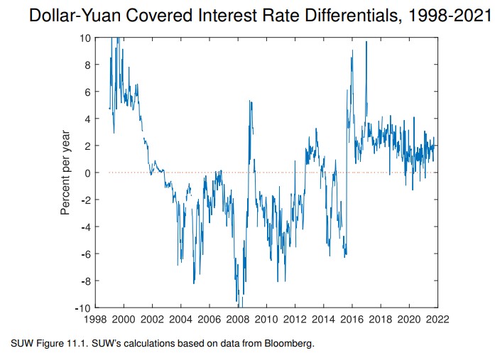
• There are large deviations from covered interest parity (3.1 percentage points on average)
• In the last 5 years of the sample, the CID fell to 2.1 percentage points on average (still sizable)
• Large CIDs are a sign of impediments to capital flows
• A negative CID indicates impediments to capital inflows into China
  • Chinese wanting to borrow from abroad to invest at home but not being able to
• A positive CID indicates impediments to capital outflows from China to the U.S.
  • Chinese wanting to save abroad but not being able to

Uncovered Interest Rate Parity (UIP)

Start from the CIP equation $(1 + i_t) = (1 + i_t^*) \frac{F_t}{\varepsilon_t}$

• Replace the forward rate $F_t$ with the expected spot exchange rate $E_t(\varepsilon_{t+1})$
• This yields the uncovered interest rate parity equation

Uncovered Interest Rate Parity: If $(1 + i_t) = (1 + i_t^*)\frac{E_t(\varepsilon_{t+1})}{\varepsilon_t}$ then we say that uncovered interest rate parity (UIP) holds

• Even under free capital mobility, UIP might not hold
• This is because $F_t = E_t (\varepsilon_{t+1})$ does not always hold (both in theory and in the data)

Forward Premium Puzzle

• The so-called forward premium puzzle indicates that UIP is strongly rejected by the data:
• Conditional on CIP holding, UIP holds if and only if $E_t\frac{\varepsilon_{t+1}}{\varepsilon_t} = \frac{F_t}{\varepsilon_t}$
  • If $F_t > \varepsilon_t$ we say that the foreign currency is at a premium in the forward market
  • If UIP holds then the domestic currency is expected to depreciate when the foreign currency trades at a premium in the forward market
• CIP holds pretty well in the data.
• Thus, if UIP holds as well then the OLS regression $\frac{\varepsilon_{t+1}}{\varepsilon_t} = a + b\frac{F_t}{\varepsilon_t} + \mu_{t+1}$ should yield $a = 0$ and $b = 1$
• However, e.g., Burnside (2018) estimates $a = 0.00055$ and $b = -0.75$ as cross-country average estimates of the USD against currencies of 10 industrialized countries for January 1976 - March 2018.
• This forward premium puzzle indicates UIP is strongly rejected by the data.

Offshore-Onshore Interest Rate Differentials

Eurocurrency deposits are foreign currency deposits in a market other than the home market of the foreign currency

• e.g.: eurodollar deposits = dollar deposits outside the U.S.

offshore-onshore interest rate differential = $i_t^* - i_t$

• $i_t^*$: offshore interest rate in period t on a USD deposit
• $i_t$: onshore interest rate in period t on a USD deposit

Under free capital mobility, the offshore-onshore differential should be zero.

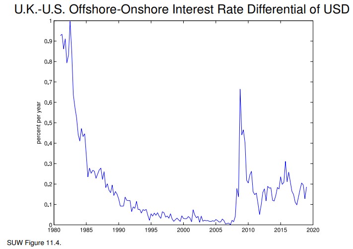
This indicates:

• free capital mobility during 1990-2008
  • Near zero offshore-onshore differential
• impediments in the 1980s and post 2008
  • attributed to post-GFC regulations
  • prevent financial institutions to exploit the
• arbitrage opportunities

The Real Interest Rate Differential

Can the real interest rate differential $r_t - r_t^*$ be a measure of free capital mobility?

Short Answer: In general, not a good measure

Consider a two-period small open economy with free capital mobility and two assets:

• $b_1$ = units of a domestic real bond
  • 1 unit pays $(1 + r_1)$ domestic consumption baskets in $t = 2$
• $b_1^*$ = units of a foreign real bond
  • 1 unit pays $(1 + r_1^*)$ foreign consumption baskets in $t = 2$

Real exchange rate: $\varepsilon_t = \frac{\varepsilon_t P_t^*}{P_t}$

Budget constraint in period 1: $C_1 + b_1 + e_1 b_1^* = Q_1$ (1)

Budget constraint in period 2: $C_2 = (1 + r_1)b_1 + (1 + r_1^*)e_2b_1^* + Q_2$ (2)

Utility: $U(C_1) + U(C_2)$

Household's optimization problem:

• $\max_{C_1, C_2} U(C_1) + U(C_2)$ s.t. (1) & (2),
• $\max_{b_1, b_1^*} U(Q_1 - b_1 - e_1b_1^*) + U((1 + r_1)b_1 + (1 + r_1^*)e_2b_1^* + Q_2)$

FOCs:

• $-U'(C_1) + (1 + r_1)U'(C_2) = 0$
• $-e_1U'(C_1) + (1 + r_1^*)e_2U'(C_2) = 0$

Solving each FOC for $\frac{U'(C_1)}{U'(C_2)}$ and equating the results yields: $(1 + r_1) = (1 + r_1^*) \frac{e_2}{e_1}$

Thus despite free capital mobility, real interest rate parity fails as long as $\frac{e_2}{e_1} \neq 1$.

L12 - Inflationary Finance & BoP Crises

How sustained fiscal deficits combined with a currency peg can end in a balance of payment crisis.

Fiscal Deficits, Inflation, and the Exchange Rate Model

a model with the following building blocks:

• more than 2 periods
• an interest-elastic demand for money
• purchasing power parity
• interest rate parity
• the government budget constraint

Demand and Supply for Money

We assume that households have a demand for money

• Money is non-interest-bearing
• People still hold money (medium of exchange)

Period-t money demand function: $\frac{M^d_t}{P_t} = L(C_t, i_t)$

• where L is a liquidity preference function
• L is increasing in period-t consumption $C_t$
• L is decreasing in the nominal interest rate $i_t$
  • The nominal interest rate $i_t$ on interest-bearing liquid assets (time deposits, ...) is the opportunity cost of holding money

We assume that $C_t = C$ for all t, thus $\frac{M^d_t}{P_t} = L(C, i_t)$

• $M_t$ denotes the nominal supply of money

The equilibrium condition in the money market is $\frac{M_t}{P_t} = L(C, i_t)$ (1)

Purchasing Power Parity

There is a single tradable good

Absolute purchasing power parity holds: $P_t = \varepsilon_t P_t^*$

For simplicity, we assume $P_t^* = 1$ for all t. Thus $P_t = \varepsilon_t$ and money market clearing condition (1) becomes: $\frac{M_t}{\varepsilon_t} = L(C, i_t)$

Interest Parity Condition

Let $i_t^*$ denote the foreign nominal interest rate in period t

• We assume that $i_t^* = i^*$ for all t
• We assume that there is free capital mobility
• We assume that there is no uncertainty
  • E.g., at time t the HH knows the entire future path of nominal exchange rates $(\varepsilon_t, \varepsilon_{t+1}, \varepsilon_{t+2}, ...)$
• We then get the interest parity condition: $1 + i_t = (1 + i_t^*) \frac{\varepsilon_{t+1}}{\varepsilon_t}$

There can be no arbitrage opportunity between domestic ($) and foreign (€) bonds

• Gross return of investing $1 in a domestic bond: $(1 + i_t)$
• Gross return of investing $1 in a foreign bond: $(1 + i_t^*) \frac{\varepsilon_{t+1}}{\varepsilon_t}$
  • $1 buys €$\frac{1}{\varepsilon_t}$ in period t
  • Investing €$\frac{1}{\varepsilon_t}$ in foreign bonds pays €$(1 + i_t^*) \frac{1}{\varepsilon_t}$ in period t + 1
  • €$(1 + i_t^*) \frac{1}{\varepsilon_t}$ buy $((1 + i_t^*) \frac{\varepsilon_{t+1}}{\varepsilon_t})$ in period t + 1

Government Budget Constraint

The period t government budget constraint is:

$\varepsilon_t B_t^g + P_t G_t = (1 + i^*) \varepsilon_t B_{t-1}^g + P_t T_t + (M_t - M_{t-1})$

• Government consumption $G_t$ and tax revenue $T_t$ are measured in units of goods
• $(M_t - M_{t-1})$ is income from money creation

Dividing by $P_t$ and rearranging yields:

$B_t^g = B_{t-1}^g + \frac{M_t - M_{t-1}}{P_t} - (G_t - T_t - i^* B_{t-1}^g)$ (2)

• $\frac{M_t - M_{t-1}}{P_t}$: seignorage revenue
• $(G_t - T_t - i^* B_{t-1}^g)$: secondary fiscal deficit

Let $DEF_t = (G_t - T_t) - i^* B_{t-1}^g$

Then, using $P_t = \varepsilon_t$, we have:

$B_t^g = B_{t-1}^g + \frac{M_t - M_{t-1}}{\varepsilon_t} - DEF_t$ (3)

If $DEF_t > 0$, then:

• the government creates money ($M_t - M_{t-1} > 0$) and/or
• the government's asset position declines ($B_t^g < B_{t-1}^g$)

Fiscal Deficits and the Sustainability of Currency Pegs

First, consider a fixed exchange rate regime:

• $\varepsilon_t = \varepsilon$ for all t
• Government intervenes in the forex market to keep $\varepsilon$ fixed
• Money supply $M_t$ becomes an endogenous variable because the central bank must stand ready to exchange domestic for foreign currency at the fixed rate $\varepsilon$

By PPP:

• $P_t = \varepsilon$ for all t
• stop high inflation -> pegging its currency to a low-inflation country
  • Argentina did that in 1991 by pegging the peso to the USD
• exchange rate-based stabilization program is however only a short-lived remedy to high inflation if not accompanied by fiscal reform

By the interest parity condition: $i_t = i^*$

Money market clearing condition: $M_t = \varepsilon L(C, i^*)$

• Money supply is constant in equilibrium
• Revenue from seignorage is zero

The government budget constraint simplifies to:

$B_t^g = B_{t-1}^g + \frac{M_t - M_{t-1}}{\varepsilon} - DEF_t = B_{t-1}^g - DEF_t$

• Fiscal deficit is financed by running down government asset holdings

Suppose that:

• there is an upper limit on the size of the public debt $B_t^g \geq D$ for all t, where D ≤ 0 is the debt limit
• $DEF_t = DEF > 0$ for all t

Then at some point, to avoid $B_t^g < D$, the government must:

• reduce its fiscal deficit (e.g. $DEF_t = 0$ for all t ≥ T) OR
• default on its debt OR
• abandon the currency peg

Such a situation is called a balance of payments crisis

Fiscal Consequences of an Unexpected Devaluation

Scenario: Suppose that in period t the central bank unexpectedly devalues the currency

• $\varepsilon_{t-1} = \varepsilon$ but $\varepsilon_t = \varepsilon ' > \varepsilon$

By PPP, $P_{t-1} = \varepsilon$ and $P_t = \varepsilon '$

• The devaluation causes inflation

By interest parity, $i_{t-1} = i_t = i^*$:

• In every period the HH expects the nominal exchange rate to remain unchanged:
  • In t - 1, the HH (wrongly) expects that $\varepsilon_{t-1} = \varepsilon_t = \varepsilon$
  • In t, the HH expects $\varepsilon_t = \varepsilon_{t+1} = \varepsilon '$

The demand for nominal money balances increases from $M_{t-1}^d = \varepsilon L(C, i^*)$ to $M_t^d = \varepsilon 'L(C, i^*)$

The period-t government budget constraint becomes:

$B_t^g = B_{t-1}^g + \frac{M_t - M_{t-1}}{\varepsilon_t} - DEF_t$

$B_t^g = B_{t-1}^g + \frac{\varepsilon 'L(C, i^*) - \varepsilon L(C, i^*)}{\varepsilon '} - DEF$

• $\frac{\varepsilon 'L(C, i^*) - \varepsilon L(C, i^*)}{\varepsilon '} > 0$

A surprise devaluation increases government revenue in the period in which the devaluation takes place

Seignorage reverts to zero in period t + 1 as the exchange rate remains constant and equal to $\varepsilon '$ from then on

Inflationary Finance of Fiscal Deficits

Next, consider a floating exchange rate regime in which the central bank targets a path for the money supply

Specifically, suppose that $M_t = (1 + \mu)M_{t-1}, \forall t = 1, 2, \ldots$, where $\mu > 0$ is the growth rate of money supply

Verify that: $\frac{\varepsilon_{t+1}}{\varepsilon_t} = (1 + \mu), \forall t = 1, 2, \ldots$

By PPP: $\frac{P_{t+1}}{P_t} = (1 + \mu), \forall t = 1, 2, \ldots$

• Inflation equals the growth rate of the money supply

By interest parity: $1 + i_t = (1 + i^*)\frac{\varepsilon_{t+1}}{\varepsilon_t} = (1 + i^*)(1 + \mu), \forall t = 1, 2, \ldots$ (4)

• Let $i(\mu) = (1 + i^*)(1 + \mu) - 1$ denote the solution to (4)
• Observe $i(\mu)$ is increasing in $\mu$

From money market clearing: $\frac{M_t}{\varepsilon_t} = L(C, i(\mu)), \forall t = 1, 2, \ldots$, we infer that

$\varepsilon_{t+1} = \frac{M_{t+1}}{L(C, i(\mu))} = \frac{(1 + \mu)M_t}{L(C, i(\mu))} = (1 + \mu)\varepsilon_t, \forall t = 1, 2, \ldots$

Conclusion:

• The nominal exchange rate grows at the same rate as money supply
• Real money balances in equilibrium are constant and decreasing in $\mu$

From $M_t = \varepsilon_tL(C, i(\mu)), \forall t = 1, 2, \ldots$, we obtain:

$\frac{M_t - M_{t-1}}{\varepsilon_t} = \frac{\varepsilon_tL(C, i(\mu)) - \varepsilon_{t-1}L(C, i(\mu))}{\varepsilon_t}$

$\frac{M_t - M_{t-1}}{\varepsilon_t} = \frac{\varepsilon_t - \varepsilon_{t-1}}{\varepsilon_t}L(C, i(\mu))$

$\frac{M_t - M_{t-1}}{\varepsilon_t} = \frac{\varepsilon_{t-1}(1 + \mu) - \varepsilon_{t-1}}{\varepsilon_{t-1}(1 + \mu)}L(C, i(\mu))$

$\frac{M_t - M_{t-1}}{\varepsilon_t} = \frac{\mu}{1 + \mu}L(C, i(\mu))$ (inflation tax revenue)

Growing money supply at a constant rate creates seignorage revenue.

Inflationary Finance and the Laffer Curve of Inflation

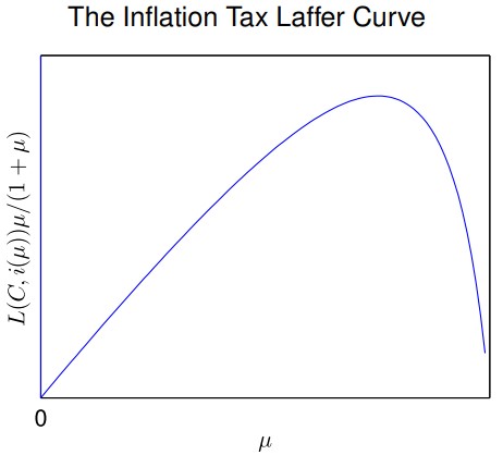
Typically, inflation tax revenue as a function of µ has an “inverted U” shape.

Suppose that the government finances a constant fiscal deficit entirely through seignorage revenue

• $DEF_t = DEF > 0$ for all t
• $B_t^g = B_{t-1}^g$ for all t (e.g. because the government reached its borrowing limit)
• The government finances the fiscal deficit by printing money (monetization of the fiscal deficit)

Then the government budget constraint simplifies to:

$DEF = \frac{M_t - M_{t-1}}{\varepsilon_t} = \frac{\mu}{1 + \mu}L(C, i(\mu))$

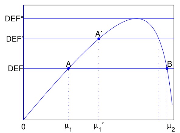
There are 2 values of the money growth rate, $\mu_1$ and $\mu_2$, that generate enough seignorage revenue to finance $DEF$.

We assume $DEF$ is financed by $\mu_1$ (point A).

• Typically, economies are on the upward-sloping part of their Laffer curve

An increase in the fiscal deficit from $DEF$ to $DEF'$ requires increasing the money supply at a faster rate (point A').

• This implies a higher inflation of $\mu'$ and a higher depreciation rate of $\mu'$

Deficits above $DEF^*$ cannot be solely financed by printing money

Balance of Payments (BOP) Crisis

Suppose the government pegs the nominal exchange
rate and runs fiscal deficits $DEF_t ≥ DEF > 0$:

• unsustainable & BOP Crisis
• the central bank often suffers a speculative attack
  • right before the peg is abandoned
  • loses vast amounts of foreign reserves in a short period of time

BOP Crisis Model Setup:

• Government runs a fiscal deficit of $DEF > 0$ each period
• announces a currency peg in period 1
  • The government fixes the nominal exchange rate: $\varepsilon_t = \varepsilon$
• initially holds a positive stock of foreign assets: $B_0^g > 0$
  • Think of $B_0^g$ as foreign reserves
• has no access to credit, i.e. faces the borrowing constraints $B_t^g \geq 0, \forall t = 1, 2, \ldots$

Technical assumptions:

• $M_0 = \varepsilon L(C, i^*)$
• $B_0^g$ equals $(L(C, i^*) - L(C, i(\mu)))$ plus a multiple of $DEF$

3 phases of a BOP crisis:

• Pre-Crisis Phase: periods $t \leq T - 2$
  • currency pegged and expected to be pegged in the next period
• BOP Crisis: period $T - 1$
  • currency pegged but peg is expected to be abandoned in the next period
  • speculative attack
• Post-Crisis Phase: periods $t \geq T$
  • currency no longer pegged
  • government ran out of foreign reserves
  • government prints money to finance its fiscal deficit

Pre-Crisis Phase

Pre-Crisis Phase: $t \in \{1, \ldots, T - 2\}$

The currency is pegged in the current and next period: $\varepsilon_t = \varepsilon_{t+1} = \varepsilon$

Therefore:

• $P_t = \varepsilon$
• $i_t = i^*$
• $M_t = \varepsilon L(C, i^*)$
• Seignorage is $\frac{M_t - M_{t-1}}{P_t} = 0$
• The central bank loses foreign reserves: $B_t^g = B_{t-1}^g - DEF$

Post-Crisis Phase

Post-Crisis Phase: $t \in \{T, T + 1, \ldots\}$

• $B_{t-1}^g = B_t^g = 0$ (the government has no foreign reserves)
• government prints money at rate $\mu$ to finance fiscal deficit: $M_t = (1 + \mu)M_{t-1}$
• $\varepsilon_t = (1 + \mu)\varepsilon_{t-1}$
• $P_t = (1 + \mu)P_{t-1}$
• $1 + i_t = (1 + \mu)(1 + i^*)$ or $i_t = i(\mu)$
• $M_t = P_tL(C, i(\mu))$
• seignorage $\frac{M_t - M_{t-1}}{P_t} = L(C, i(\mu))\frac{\mu}{1 + \mu}$
• $DEF = L(C, i(\mu))\frac{\mu}{1 + \mu}$

BOP Crisis Phase

BOP Crisis: period $T - 1$

The currency peg is in place but about to collapse: $\varepsilon_{T-1} = \varepsilon < \varepsilon_T$

How large is the depreciation between $T - 1$ and $T$?

The government budget constraint for $t = T$:

$L(C, i(\mu))(1 - \frac{1}{1 + \mu}) = DEF = \frac{M_T - M_{T-1}}{\varepsilon_T} = \frac{M_T}{\varepsilon_T} - \frac{M_{T-1}}{\varepsilon_{T-1}}\frac{\varepsilon_{T-1}}{\varepsilon_T} = L(C, i(\mu)) - \frac{M_{T-1}}{\varepsilon_{T-1}}\frac{\varepsilon_{T-1}}{\varepsilon_T}$

The above implies:

$L(C, i(\mu))\frac{1}{1 + \mu} = \frac{M_{T-1}}{\varepsilon_{T-1}}\frac{\varepsilon_{T-1}}{\varepsilon_T}$ (5)

Money market clearing in $T - 1$ implies:

$\frac{M_{T-1}}{\varepsilon_{T-1}} = L(C, i_{T-1})$

interest parity for bonds purchased in $T - 1$ implies:

$\frac{\varepsilon_{T-1}}{\varepsilon_T} = \frac{1+i^*}{1+i_{T-1}}$ (6)

Plugging these into (5) yields:

$\frac{1}{1 + \mu} = L(C, i_{T-1}) \frac{1+i^*}{1+i_{T-1}}$ (7)

$i_{T-1} = i(\mu)$ solves (7) because $\frac{1+i^*}{1+(1/\mu)} = \frac{1}{1+\mu}$

Moreover, only $i_{T-1} = i(\mu)$ solves (7) because both $L(C, i_{T-1})$ and $\frac{1+i^*}{1+i_{T-1}}$ are decreasing in $i_{T-1}$

Thus in $T - 1$:

• the nominal interest rate increases to its post-crisis level $i(\mu)$
• real balances $\frac{M_t}{\varepsilon_t}$ fall to their post-crisis level $L(C, i(\mu))$

Finally, $i_{T-1} = i(\mu)$ and (6) imply that the rate of currency depreciation between $T - 1$ & $T$ is $\mu$:

$\varepsilon_T = (1 + \mu)\varepsilon_{T-1}$

Seignorage equals:

$\frac{M_{T-1} - M_{T-2}}{\varepsilon_{T-1}} = \frac{M_{T-1}}{\varepsilon_{T-1}} - \frac{M_{T-2}}{\varepsilon_{T-1}} = L(C, i(\mu)) - \frac{eL(C, i^*)}{e}$

Foreign reserves of the central bank fall by more than $DEF$:

$B_{T-1}^g = B_{T-2}^g + \frac{M_{T-1} - M_{T-2}}{\varepsilon_{T-1}} - DEF$

$B_{T-1}^g = B_{T-2}^g + L(C, i(\mu)) - L(C, i^*) - DEF$

$B_{T-1}^g < B_{T-2}^g - DEF$

Note that $L(C, i(\mu)) - L(C, i^*) < 0$

The Dynamics of a Balance of Payments Crisis

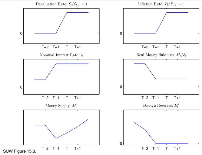
• The depreciation rate and inflation are zero until $T - 1$ and jump to a permanently higher level in $T$
• The nominal interest rate jumps one period earlier in $T - 1$ because of the anticipated depreciation in $T$
• The increase in the interest rate induces households to reduce their real money holdings in $T - 1$
• Nominal money demand $M^d_t = \varepsilon_tL(C, i)$ and thus nominal money supply $M_t$
  • drop in $T - 1$ as $i_{T-1} > i_{T-2}$ while $\varepsilon_{T-1} = \varepsilon$
  • grow at a constant rate from $T$ on (creating seignorage)
• Foreign reserves fall by $DEF$ per period until $T - 2$ and then get depleted by a final, larger drop in $T - 1$

Epilogue

这些东西学得也太费劲了

第一次尝试在 markdown 中插入这么多公式，手机上可能性能不够，加载时间比较长。。。

公式当然不是手敲的，前期使用了 lukas-blecher/LaTeX-OCR 这个项目，后期使用 ChatGPT 4 进行 OCR。